

8 Chain Rule Optimal Transport
195
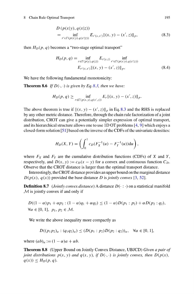
D ( p(x|y), q(x|z))
=
inf
r ∈( p(x|y),q(x |z))
E r (x,x ) (x, y) − (x
, z) p ,
(8.3)
then H D ( p, q) becomes a “two-stage optimal transport”
H D ( p, q) =
inf
r ∈( p(y),q(z))
E r (y,z)
inf
r ∈( p(x|y),q(x |z))
E r (x,x ) (x, y) − (x
, z) p ,
(8.4)
We have the following fundamental monotonicity:
Theorem 8.6 If D(·, ·) is given by Eq. 8.3, then we have:
H D ( p, q) ≥
inf
r ∈( p(x,y),q(x ,z))
E r (x, y) − (x
, z) p .
The above theorem is true if (x, y) − (x
, z) p in Eq. 8.3 and the RHS is replaced
by any other metric distance. Therefore, through the chain rule factorization of a joint
distribution, CROT can give a potentially simpler expression of optimal transport,
and its hierarchical structure allows one to use 1D OT problems [4, 9] which enjoys a
closed-form solution [51] based on the inverse of the CDFs of the univariate densities:
H D (X, Y ) =
1
0
c D (F
−1
X (u) − F
−1
Y (u))du
,
where F X and F Y are the cumulative distribution functions (CDFs) of X and Y ,
respectively, and D(x, y) := c D (x − y) for a convex and continuous function C D .
Observe that the CROT distance is larger than the optimal transport distance.
Interestingly, the CROT distance provides an upper bound on the marginal distance
D( p(x), q(x)) provided the base distance D is jointly convex [3, 52].
Definition 8.7 (Jointly convex distance) A distance D(· : ·) on a statistical manifold
M is jointly convex if and only if
D((1 − α) p 1 + αp 2 : (1 − α)q 1 + αq 2 ) ≤ (1 − α)D( p 1 : p 2 ) + α D( p 2 : q 2 ),
∀α ∈ [0, 1], p 1 , p 2 ∈ M.
We write the above inequality more compactly as
D(( p 1 p 2 ) α : (q 1 q 2 ) α ) ≤ (D( p 1 : p 2 )D( p 2 : q 2 )) α , ∀α ∈ [0, 1],
where (ab) α := (1 − α)a + αb.
Theorem 8.8 (Upper Bound on Jointly Convex Distance, UBJCD) Given a pair of
joint distributions p(x, y) and q(x, y), if D(·, ·) is jointly convex, then D( p(x),
q(x)) ≤ H D ( p, q).
195
D ( p(x|y), q(x|z))
=
inf
r ∈( p(x|y),q(x |z))
E r (x,x ) (x, y) − (x
, z) p ,
(8.3)
then H D ( p, q) becomes a “two-stage optimal transport”
H D ( p, q) =
inf
r ∈( p(y),q(z))
E r (y,z)
inf
r ∈( p(x|y),q(x |z))
E r (x,x ) (x, y) − (x
, z) p ,
(8.4)
We have the following fundamental monotonicity:
Theorem 8.6 If D(·, ·) is given by Eq. 8.3, then we have:
H D ( p, q) ≥
inf
r ∈( p(x,y),q(x ,z))
E r (x, y) − (x
, z) p .
The above theorem is true if (x, y) − (x
, z) p in Eq. 8.3 and the RHS is replaced
by any other metric distance. Therefore, through the chain rule factorization of a joint
distribution, CROT can give a potentially simpler expression of optimal transport,
and its hierarchical structure allows one to use 1D OT problems [4, 9] which enjoys a
closed-form solution [51] based on the inverse of the CDFs of the univariate densities:
H D (X, Y ) =
1
0
c D (F
−1
X (u) − F
−1
Y (u))du
,
where F X and F Y are the cumulative distribution functions (CDFs) of X and Y ,
respectively, and D(x, y) := c D (x − y) for a convex and continuous function C D .
Observe that the CROT distance is larger than the optimal transport distance.
Interestingly, the CROT distance provides an upper bound on the marginal distance
D( p(x), q(x)) provided the base distance D is jointly convex [3, 52].
Definition 8.7 (Jointly convex distance) A distance D(· : ·) on a statistical manifold
M is jointly convex if and only if
D((1 − α) p 1 + αp 2 : (1 − α)q 1 + αq 2 ) ≤ (1 − α)D( p 1 : p 2 ) + α D( p 2 : q 2 ),
∀α ∈ [0, 1], p 1 , p 2 ∈ M.
We write the above inequality more compactly as
D(( p 1 p 2 ) α : (q 1 q 2 ) α ) ≤ (D( p 1 : p 2 )D( p 2 : q 2 )) α , ∀α ∈ [0, 1],
where (ab) α := (1 − α)a + αb.
Theorem 8.8 (Upper Bound on Jointly Convex Distance, UBJCD) Given a pair of
joint distributions p(x, y) and q(x, y), if D(·, ·) is jointly convex, then D( p(x),
q(x)) ≤ H D ( p, q).