

182
F. Nielsen
Remember that the intersection of θ -flats is a θ -flat.
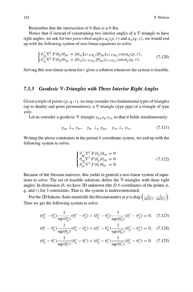
Notice that if instead of constraining two interior angles of a ∇-triangle to have
right angles, we ask for two prescribed angles α q ( p, r ) and α p (q, r ), we would end
up with the following system of non-linear equations to solve:
θ
rq ∇
2 F(θ q )θ pq = =θ rq ∇ 2 F(θ q ) θ pq ∇ 2 F(θ q ) cos α q ( p, r ),
θ
rq ∇
2 F(θ p )θ pq = =θ rq | ∇ 2 F(θ p ) θ pq | ∇ 2 F(θ p ) cos α p (q, r ).
(7.120)
Solving this non-linear system for r gives a solution whenever the system is feasible.
7.3.3 Geodesic ∇-Triangles with Three Interior Right Angles
Given a triple of points ( p, q, r ), we may consider two fundamental types of triangles
(up to duality and point permutations): a ∇-triangle (type ppp) or a triangle of type
pdp.
Let us consider a geodesic ∇-triangle γ pq γ qr γ r p so that it holds simultaneously:
γ pq ⊥ p γ pr , γ qr ⊥ q γ qp , γ r p ⊥ r γ rq .
(7.121)
Writing the above constraints in the primal θ -coordinate system, we end up with the
following system to solve:
⎧
⎨
⎩
θ
qp ∇
2 F(θ p )θ r p = 0
θ
rq ∇
2 F(θ q )θ pq = 0
θ
pr ∇
2 F(θ r )θ qr = 0.
(7.122)
Because of the Hessian matrices, this yields in general a non-linear system of equations to solve. The set of feasible solutions define the ∇-triangles with three right
angles. In dimension D, we have 3D unknown (the D θ -coordinates of the points p,
q, and r ) for 3 constraints. That is, the system is underconstrained.
For the 2D Itakura–Saito manifold, the Hessian matrix at p is diag
1
sqr(θ x )
,
1
sqr(θ y )
.
Thus we get the following system to solve:
(θ
x
q − θ
x
p )
1
sqr(θ x
p )
(θ
x
r − θ
x
p ) + (θ
y
q − θ
y
p )
1
sqr(θ
y
p )
(θ
y
r − θ
y
p ) = 0, (7.123)
(θ
x
r − θ
x
q )
1
sqr(θ x
q )
(θ
x
p − θ
x
q ) + (θ
y
r − θ
y
q )
1
sqr(θ
y
q )
(θ
y
p − θ
y
q ) = 0, (7.124)
(θ
x
p − θ
x
r )
1
sqr(θ x
r )
(θ
x
q − θ
x
r ) + (θ
y
p − θ
y
r )
1
sqr(θ
y
r )
(θ
y
q − θ
y
r ) = 0. (7.125)
F. Nielsen
Remember that the intersection of θ -flats is a θ -flat.
Notice that if instead of constraining two interior angles of a ∇-triangle to have
right angles, we ask for two prescribed angles α q ( p, r ) and α p (q, r ), we would end
up with the following system of non-linear equations to solve:
θ
rq ∇
2 F(θ q )θ pq = =θ rq ∇ 2 F(θ q ) θ pq ∇ 2 F(θ q ) cos α q ( p, r ),
θ
rq ∇
2 F(θ p )θ pq = =θ rq | ∇ 2 F(θ p ) θ pq | ∇ 2 F(θ p ) cos α p (q, r ).
(7.120)
Solving this non-linear system for r gives a solution whenever the system is feasible.
7.3.3 Geodesic ∇-Triangles with Three Interior Right Angles
Given a triple of points ( p, q, r ), we may consider two fundamental types of triangles
(up to duality and point permutations): a ∇-triangle (type ppp) or a triangle of type
pdp.
Let us consider a geodesic ∇-triangle γ pq γ qr γ r p so that it holds simultaneously:
γ pq ⊥ p γ pr , γ qr ⊥ q γ qp , γ r p ⊥ r γ rq .
(7.121)
Writing the above constraints in the primal θ -coordinate system, we end up with the
following system to solve:
⎧
⎨
⎩
θ
qp ∇
2 F(θ p )θ r p = 0
θ
rq ∇
2 F(θ q )θ pq = 0
θ
pr ∇
2 F(θ r )θ qr = 0.
(7.122)
Because of the Hessian matrices, this yields in general a non-linear system of equations to solve. The set of feasible solutions define the ∇-triangles with three right
angles. In dimension D, we have 3D unknown (the D θ -coordinates of the points p,
q, and r ) for 3 constraints. That is, the system is underconstrained.
For the 2D Itakura–Saito manifold, the Hessian matrix at p is diag
1
sqr(θ x )
,
1
sqr(θ y )
.
Thus we get the following system to solve:
(θ
x
q − θ
x
p )
1
sqr(θ x
p )
(θ
x
r − θ
x
p ) + (θ
y
q − θ
y
p )
1
sqr(θ
y
p )
(θ
y
r − θ
y
p ) = 0, (7.123)
(θ
x
r − θ
x
q )
1
sqr(θ x
q )
(θ
x
p − θ
x
q ) + (θ
y
r − θ
y
q )
1
sqr(θ
y
q )
(θ
y
p − θ
y
q ) = 0, (7.124)
(θ
x
p − θ
x
r )
1
sqr(θ x
r )
(θ
x
q − θ
x
r ) + (θ
y
p − θ
y
r )
1
sqr(θ
y
r )
(θ
y
q − θ
y
r ) = 0. (7.125)