

7 On Geodesic Triangles with Right Angles in a Dually Flat Space
157
θ-coordinates
η-coordinates
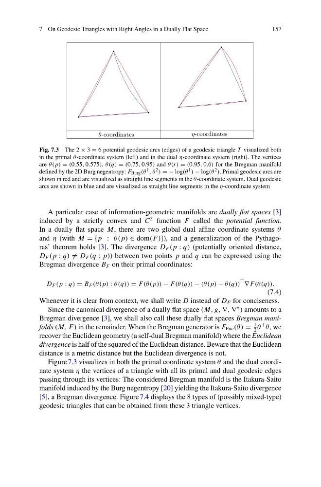
Fig. 7.3 The 2 × 3 = 6 potential geodesic arcs (edges) of a geodesic triangle T visualized both
in the primal θ-coordinate system (left) and in the dual η-coordinate system (right). The vertices
are θ( p) = (0.55, 0.575), θ(q) = (0.75, 0.95) and θ(r ) = (0.95, 0.6) for the Bregman manifold
defined by the 2D Burg negentropy: F Burg (θ 1 , θ 2 ) = − log(θ 1 ) − log(θ 2 ). Primal geodesic arcs are
shown in red and are visualized as straight line segments in the θ-coordinate system. Dual geodesic
arcs are shown in blue and are visualized as straight line segments in the η-coordinate system
A particular case of information-geometric manifolds are dually flat spaces [3]
induced by a strictly convex and C
3 function F called the potential function.
In a dually flat space M, there are two global dual affine coordinate systems θ
and η (with M = {p : θ( p) ∈ dom(F)}), and a generalization of the Pythagoras’ theorem holds [3]. The divergence D F ( p : q) (potentially oriented distance,
D F ( p : q) = D F (q : p)) between two points p and q can be expressed using the
Bregman divergence B F on their primal coordinates:
D F ( p : q) = B F (θ ( p) : θ(q)) = F(θ ( p)) − F(θ (q)) − (θ ( p) − θ(q))
∇ F(θ (q)).
(7.4)
Whenever it is clear from context, we shall write D instead of D F for conciseness.
Since the canonical divergence of a dually flat space (M, g, ∇, ∇
∗
) amounts to a
Bregman divergence [3], we shall also call these dually flat spaces Bregman manifolds (M, F) in the remainder. When the Bregman generator is F Euc (θ ) =
1
2
θ
θ , we
recover the Euclidean geometry (a self-dual Bregman manifold) where the Euclidean
divergence is half of the squared of the Euclidean distance. Beware that the Euclidean
distance is a metric distance but the Euclidean divergence is not.
Figure 7.3 visualizes in both the primal coordinate system θ and the dual coordinate system η the vertices of a triangle with all its primal and dual geodesic edges
passing through its vertices: The considered Bregman manifold is the Itakura-Saito
manifold induced by the Burg negentropy [20] yielding the Itakura-Saito divergence
[5], a Bregman divergence. Figure 7.4 displays the 8 types of (possibly mixed-type)
geodesic triangles that can be obtained from these 3 triangle vertices.
157
θ-coordinates
η-coordinates
Fig. 7.3 The 2 × 3 = 6 potential geodesic arcs (edges) of a geodesic triangle T visualized both
in the primal θ-coordinate system (left) and in the dual η-coordinate system (right). The vertices
are θ( p) = (0.55, 0.575), θ(q) = (0.75, 0.95) and θ(r ) = (0.95, 0.6) for the Bregman manifold
defined by the 2D Burg negentropy: F Burg (θ 1 , θ 2 ) = − log(θ 1 ) − log(θ 2 ). Primal geodesic arcs are
shown in red and are visualized as straight line segments in the θ-coordinate system. Dual geodesic
arcs are shown in blue and are visualized as straight line segments in the η-coordinate system
A particular case of information-geometric manifolds are dually flat spaces [3]
induced by a strictly convex and C
3 function F called the potential function.
In a dually flat space M, there are two global dual affine coordinate systems θ
and η (with M = {p : θ( p) ∈ dom(F)}), and a generalization of the Pythagoras’ theorem holds [3]. The divergence D F ( p : q) (potentially oriented distance,
D F ( p : q) = D F (q : p)) between two points p and q can be expressed using the
Bregman divergence B F on their primal coordinates:
D F ( p : q) = B F (θ ( p) : θ(q)) = F(θ ( p)) − F(θ (q)) − (θ ( p) − θ(q))
∇ F(θ (q)).
(7.4)
Whenever it is clear from context, we shall write D instead of D F for conciseness.
Since the canonical divergence of a dually flat space (M, g, ∇, ∇
∗
) amounts to a
Bregman divergence [3], we shall also call these dually flat spaces Bregman manifolds (M, F) in the remainder. When the Bregman generator is F Euc (θ ) =
1
2
θ
θ , we
recover the Euclidean geometry (a self-dual Bregman manifold) where the Euclidean
divergence is half of the squared of the Euclidean distance. Beware that the Euclidean
distance is a metric distance but the Euclidean divergence is not.
Figure 7.3 visualizes in both the primal coordinate system θ and the dual coordinate system η the vertices of a triangle with all its primal and dual geodesic edges
passing through its vertices: The considered Bregman manifold is the Itakura-Saito
manifold induced by the Burg negentropy [20] yielding the Itakura-Saito divergence
[5], a Bregman divergence. Figure 7.4 displays the 8 types of (possibly mixed-type)
geodesic triangles that can be obtained from these 3 triangle vertices.