

3.2
0.22
Speed (m/s)
2
4
6
8
10
1.0 2.0 3.0 4.0 5.0 6.0 7.0 8.0
Locomotion Curvature
2.4
1.6
0.16
0.10
0.04
0.8
Driving Input u 0
Time Constant τ 1 (τ 1 /τ 2 = 1/3)
(a)
(b)
23
CPG-Based Control of Serpentine Locomotion of a Snake-Like Robot
TABLE 2.3
Physical Parameters of the Simulated Robot
Numbers of joints
Num = 10
Length of link
L link = 0.13 m
Radius of link
R link = 0.02 m
Weight of link
M link = 0.2 kg
Width of wheel
L wheel = 0.01 m
Radius of wheel
R wheel = 0.03 m
Weight of wheel
M wheel = 0.08 kg
Friction coefficients
μ N = 0.5, μ T = 0.02
on the ith joint as the angle input signal. Each angle of the robot joint θ i can
be calculated by
θ i = α i y o u t i
(2.8)
where α i is a gain from the control signal to the joint angle. Here, each α i
takes the same value due to the uniform CPG output (the value of α i was
considered as 1.0 with respect to the set of parameters in Table 2.1).
2.4.1 Control of the Locomotion Curvature
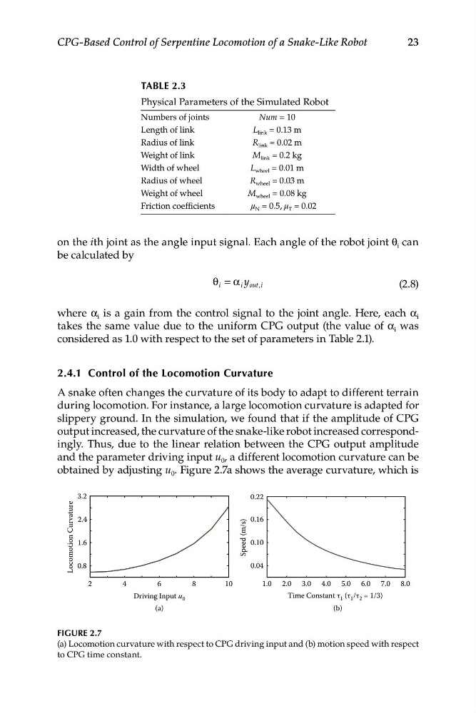
A snake often changes the curvature of its body to adapt to different terrain
during locomotion. For instance, a large locomotion curvature is adapted for
slippery ground. In the simulation, we found that if the amplitude of CPG
output increased, the curvature of the snake-like robot increased correspondingly. Thus, due to the linear relation between the CPG output amplitude
and the parameter driving input u 0 , a different locomotion curvature can be
obtained by adjusting u 0 . Figure 2.7a shows the average curvature, which is
FIGURE 2.7
(a) Locomotion curvature with respect to CPG driving input and (b) motion speed with respect
to CPG time constant.
0.22
Speed (m/s)
2
4
6
8
10
1.0 2.0 3.0 4.0 5.0 6.0 7.0 8.0
Locomotion Curvature
2.4
1.6
0.16
0.10
0.04
0.8
Driving Input u 0
Time Constant τ 1 (τ 1 /τ 2 = 1/3)
(a)
(b)
23
CPG-Based Control of Serpentine Locomotion of a Snake-Like Robot
TABLE 2.3
Physical Parameters of the Simulated Robot
Numbers of joints
Num = 10
Length of link
L link = 0.13 m
Radius of link
R link = 0.02 m
Weight of link
M link = 0.2 kg
Width of wheel
L wheel = 0.01 m
Radius of wheel
R wheel = 0.03 m
Weight of wheel
M wheel = 0.08 kg
Friction coefficients
μ N = 0.5, μ T = 0.02
on the ith joint as the angle input signal. Each angle of the robot joint θ i can
be calculated by
θ i = α i y o u t i
(2.8)
where α i is a gain from the control signal to the joint angle. Here, each α i
takes the same value due to the uniform CPG output (the value of α i was
considered as 1.0 with respect to the set of parameters in Table 2.1).
2.4.1 Control of the Locomotion Curvature
A snake often changes the curvature of its body to adapt to different terrain
during locomotion. For instance, a large locomotion curvature is adapted for
slippery ground. In the simulation, we found that if the amplitude of CPG
output increased, the curvature of the snake-like robot increased correspondingly. Thus, due to the linear relation between the CPG output amplitude
and the parameter driving input u 0 , a different locomotion curvature can be
obtained by adjusting u 0 . Figure 2.7a shows the average curvature, which is
FIGURE 2.7
(a) Locomotion curvature with respect to CPG driving input and (b) motion speed with respect
to CPG time constant.