

271
Mathematical Modeling of Brain Circuitry
& = ⎡ ⎣ 20 5466 − .
4 4225
.
5 8488 ⎤ ⎦
.
9 6495
.
1 8089
.
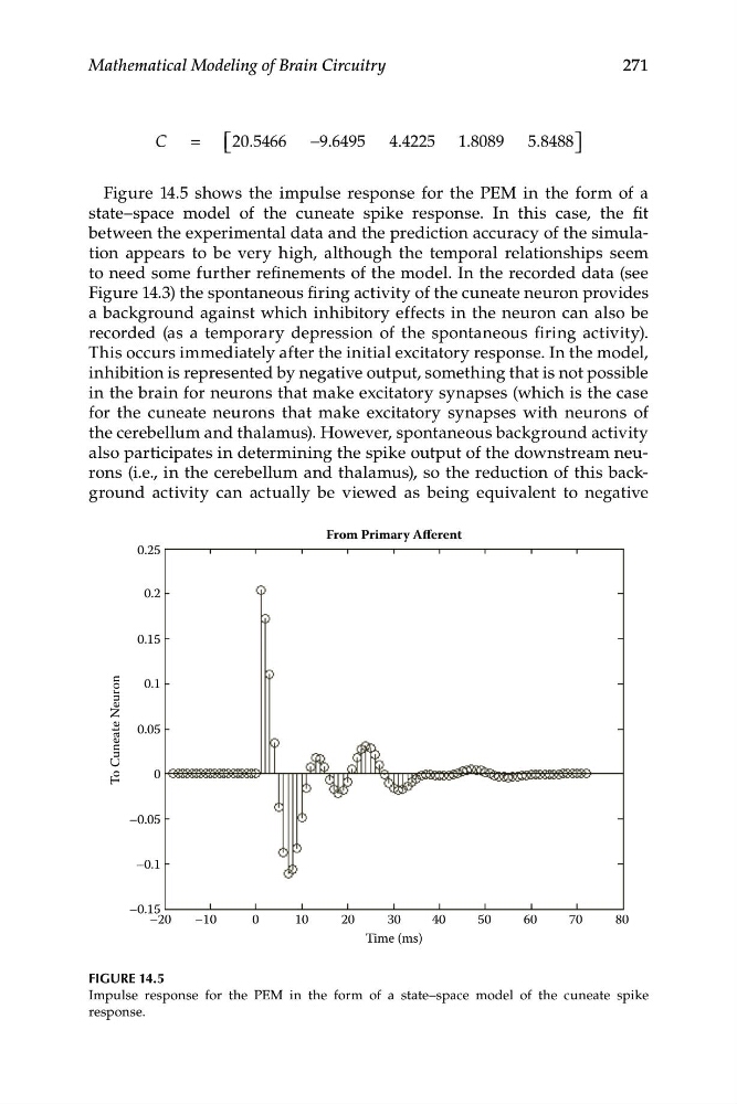
Figure 14.5 shows the impulse response for the PEM in the form of a
state–space model of the cuneate spike response. In this case, the fit
between the experimental data and the prediction accuracy of the simulation appears to be very high, although the temporal relationships seem
to need some further refinements of the model. In the recorded data (see
Figure 14.3) the spontaneous firing activity of the cuneate neuron provides
a background against which inhibitory effects in the neuron can also be
recorded (as a temporary depression of the spontaneous firing activity).
This occurs immediately after the initial excitatory response. In the model,
inhibition is represented by negative output, something that is not possible
in the brain for neurons that make excitatory synapses (which is the case
for the cuneate neurons that make excitatory synapses with neurons of
the cerebellum and thalamus). However, spontaneous background activity
also participates in determining the spike output of the downstream neurons (i.e., in the cerebellum and thalamus), so the reduction of this background activity can actually be viewed as being equivalent to negative
0.25
0.2
0.15
0.1
0.05
0
–0.05
–0.1
–0.15
From Primary Afferent
–20
–10
0
10
20
30
40
5 0
6 0
7 0
8 0
To Cuneate Neuron
Time (ms)
FIGURE 14.5
Impulse response for the PEM in the form of a state–space model of the cuneate spike
response.
Mathematical Modeling of Brain Circuitry
& = ⎡ ⎣ 20 5466 − .
4 4225
.
5 8488 ⎤ ⎦
.
9 6495
.
1 8089
.
Figure 14.5 shows the impulse response for the PEM in the form of a
state–space model of the cuneate spike response. In this case, the fit
between the experimental data and the prediction accuracy of the simulation appears to be very high, although the temporal relationships seem
to need some further refinements of the model. In the recorded data (see
Figure 14.3) the spontaneous firing activity of the cuneate neuron provides
a background against which inhibitory effects in the neuron can also be
recorded (as a temporary depression of the spontaneous firing activity).
This occurs immediately after the initial excitatory response. In the model,
inhibition is represented by negative output, something that is not possible
in the brain for neurons that make excitatory synapses (which is the case
for the cuneate neurons that make excitatory synapses with neurons of
the cerebellum and thalamus). However, spontaneous background activity
also participates in determining the spike output of the downstream neurons (i.e., in the cerebellum and thalamus), so the reduction of this background activity can actually be viewed as being equivalent to negative
0.25
0.2
0.15
0.1
0.05
0
–0.05
–0.1
–0.15
From Primary Afferent
–20
–10
0
10
20
30
40
5 0
6 0
7 0
8 0
To Cuneate Neuron
Time (ms)
FIGURE 14.5
Impulse response for the PEM in the form of a state–space model of the cuneate spike
response.