

Determination of Best-Fit Probability Distribution …
69
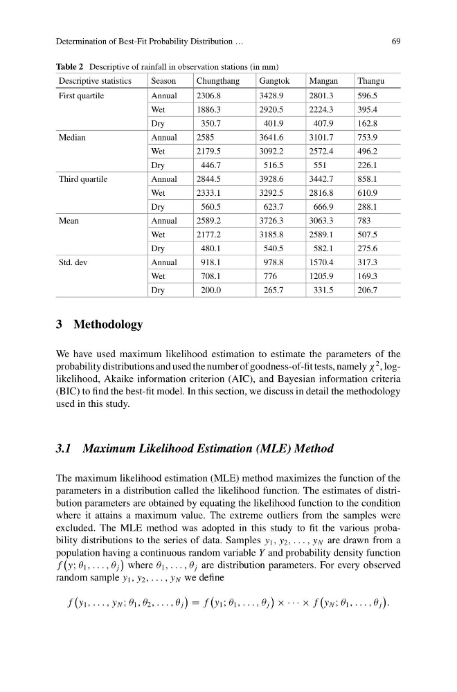
Table 2 Descriptive of rainfall in observation stations (in mm)
Descriptive statistics
Season
Chungthang
Gangtok
Mangan
Thangu
First quartile
Annual
2306.8
3428.9
2801.3
596.5
Wet
1886.3
2920.5
2224.3
395.4
Dry
350.7
401.9
407.9
162.8
Median
Annual
2585
3641.6
3101.7
753.9
Wet
2179.5
3092.2
2572.4
496.2
Dry
446.7
516.5
551
226.1
Third quartile
Annual
2844.5
3928.6
3442.7
858.1
Wet
2333.1
3292.5
2816.8
610.9
Dry
560.5
623.7
666.9
288.1
Mean
Annual
2589.2
3726.3
3063.3
783
Wet
2177.2
3185.8
2589.1
507.5
Dry
480.1
540.5
582.1
275.6
Std. dev
Annual
918.1
978.8
1570.4
317.3
Wet
708.1
776
1205.9
169.3
Dry
200.0
265.7
331.5
206.7
3 Methodology
We have used maximum likelihood estimation to estimate the parameters of the
probability distributions and used the number of goodness-of-fit tests, namely χ
2 , loglikelihood, Akaike information criterion (AIC), and Bayesian information criteria
(BIC) to find the best-fit model. In this section, we discuss in detail the methodology
used in this study.
3.1 Maximum Likelihood Estimation (MLE) Method
The maximum likelihood estimation (MLE) method maximizes the function of the
parameters in a distribution called the likelihood function. The estimates of distribution parameters are obtained by equating the likelihood function to the condition
where it attains a maximum value. The extreme outliers from the samples were
excluded. The MLE method was adopted in this study to fit the various probability distributions to the series of data. Samples y 1 , y 2 , . . . , y N are drawn from a
population having a continuous random variable Y and probability density function
f
y; θ 1 , . . . , θ j
where θ 1 , . . . , θ j are distribution parameters. For every observed
random sample y 1 , y 2 , . . . , y N we define
f
y 1 , . . . , y N ; θ 1 , θ 2 , . . . , θ j
= f
y 1 ; θ 1 , . . . , θ j
× · · · × f
y N ; θ 1 , . . . , θ j
.
69
Table 2 Descriptive of rainfall in observation stations (in mm)
Descriptive statistics
Season
Chungthang
Gangtok
Mangan
Thangu
First quartile
Annual
2306.8
3428.9
2801.3
596.5
Wet
1886.3
2920.5
2224.3
395.4
Dry
350.7
401.9
407.9
162.8
Median
Annual
2585
3641.6
3101.7
753.9
Wet
2179.5
3092.2
2572.4
496.2
Dry
446.7
516.5
551
226.1
Third quartile
Annual
2844.5
3928.6
3442.7
858.1
Wet
2333.1
3292.5
2816.8
610.9
Dry
560.5
623.7
666.9
288.1
Mean
Annual
2589.2
3726.3
3063.3
783
Wet
2177.2
3185.8
2589.1
507.5
Dry
480.1
540.5
582.1
275.6
Std. dev
Annual
918.1
978.8
1570.4
317.3
Wet
708.1
776
1205.9
169.3
Dry
200.0
265.7
331.5
206.7
3 Methodology
We have used maximum likelihood estimation to estimate the parameters of the
probability distributions and used the number of goodness-of-fit tests, namely χ
2 , loglikelihood, Akaike information criterion (AIC), and Bayesian information criteria
(BIC) to find the best-fit model. In this section, we discuss in detail the methodology
used in this study.
3.1 Maximum Likelihood Estimation (MLE) Method
The maximum likelihood estimation (MLE) method maximizes the function of the
parameters in a distribution called the likelihood function. The estimates of distribution parameters are obtained by equating the likelihood function to the condition
where it attains a maximum value. The extreme outliers from the samples were
excluded. The MLE method was adopted in this study to fit the various probability distributions to the series of data. Samples y 1 , y 2 , . . . , y N are drawn from a
population having a continuous random variable Y and probability density function
f
y; θ 1 , . . . , θ j
where θ 1 , . . . , θ j are distribution parameters. For every observed
random sample y 1 , y 2 , . . . , y N we define
f
y 1 , . . . , y N ; θ 1 , θ 2 , . . . , θ j
= f
y 1 ; θ 1 , . . . , θ j
× · · · × f
y N ; θ 1 , . . . , θ j
.