

148
S. Santra and S. Biswas
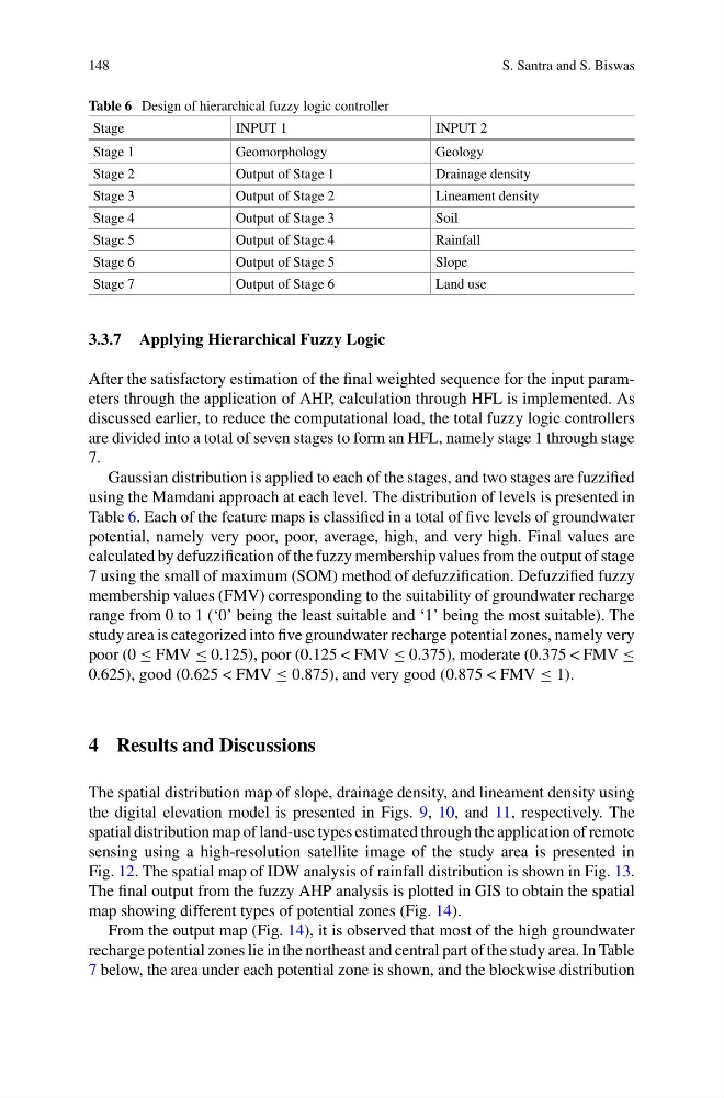
Table 6 Design of hierarchical fuzzy logic controller
Stage
INPUT 1
INPUT 2
Stage 1
Geomorphology
Geology
Stage 2
Output of Stage 1
Drainage density
Stage 3
Output of Stage 2
Lineament density
Stage 4
Output of Stage 3
Soil
Stage 5
Output of Stage 4
Rainfall
Stage 6
Output of Stage 5
Slope
Stage 7
Output of Stage 6
Land use
3.3.7 Applying Hierarchical Fuzzy Logic
After the satisfactory estimation of the final weighted sequence for the input parameters through the application of AHP, calculation through HFL is implemented. As
discussed earlier, to reduce the computational load, the total fuzzy logic controllers
are divided into a total of seven stages to form an HFL, namely stage 1 through stage
7.
Gaussian distribution is applied to each of the stages, and two stages are fuzzified
using the Mamdani approach at each level. The distribution of levels is presented in
Table 6. Each of the feature maps is classified in a total of five levels of groundwater
potential, namely very poor, poor, average, high, and very high. Final values are
calculated by defuzzification of the fuzzy membership values from the output of stage
7 using the small of maximum (SOM) method of defuzzification. Defuzzified fuzzy
membership values (FMV) corresponding to the suitability of groundwater recharge
range from 0 to 1 (‘0’ being the least suitable and ‘1’ being the most suitable). The
study area is categorized into five groundwater recharge potential zones, namely very
poor (0 ≤ FMV ≤ 0.125), poor (0.125 < FMV ≤ 0.375), moderate (0.375 < FMV ≤
0.625), good (0.625 < FMV ≤ 0.875), and very good (0.875 < FMV ≤ 1).
4 Results and Discussions
The spatial distribution map of slope, drainage density, and lineament density using
the digital elevation model is presented in Figs. 9, 10, and 11, respectively. The
spatial distribution map of land-use types estimated through the application of remote
sensing using a high-resolution satellite image of the study area is presented in
Fig. 12. The spatial map of IDW analysis of rainfall distribution is shown in Fig. 13.
The final output from the fuzzy AHP analysis is plotted in GIS to obtain the spatial
map showing different types of potential zones (Fig. 14).
From the output map (Fig. 14), it is observed that most of the high groundwater
recharge potential zones lie in the northeast and central part of the study area. In Table
7 below, the area under each potential zone is shown, and the blockwise distribution
S. Santra and S. Biswas
Table 6 Design of hierarchical fuzzy logic controller
Stage
INPUT 1
INPUT 2
Stage 1
Geomorphology
Geology
Stage 2
Output of Stage 1
Drainage density
Stage 3
Output of Stage 2
Lineament density
Stage 4
Output of Stage 3
Soil
Stage 5
Output of Stage 4
Rainfall
Stage 6
Output of Stage 5
Slope
Stage 7
Output of Stage 6
Land use
3.3.7 Applying Hierarchical Fuzzy Logic
After the satisfactory estimation of the final weighted sequence for the input parameters through the application of AHP, calculation through HFL is implemented. As
discussed earlier, to reduce the computational load, the total fuzzy logic controllers
are divided into a total of seven stages to form an HFL, namely stage 1 through stage
7.
Gaussian distribution is applied to each of the stages, and two stages are fuzzified
using the Mamdani approach at each level. The distribution of levels is presented in
Table 6. Each of the feature maps is classified in a total of five levels of groundwater
potential, namely very poor, poor, average, high, and very high. Final values are
calculated by defuzzification of the fuzzy membership values from the output of stage
7 using the small of maximum (SOM) method of defuzzification. Defuzzified fuzzy
membership values (FMV) corresponding to the suitability of groundwater recharge
range from 0 to 1 (‘0’ being the least suitable and ‘1’ being the most suitable). The
study area is categorized into five groundwater recharge potential zones, namely very
poor (0 ≤ FMV ≤ 0.125), poor (0.125 < FMV ≤ 0.375), moderate (0.375 < FMV ≤
0.625), good (0.625 < FMV ≤ 0.875), and very good (0.875 < FMV ≤ 1).
4 Results and Discussions
The spatial distribution map of slope, drainage density, and lineament density using
the digital elevation model is presented in Figs. 9, 10, and 11, respectively. The
spatial distribution map of land-use types estimated through the application of remote
sensing using a high-resolution satellite image of the study area is presented in
Fig. 12. The spatial map of IDW analysis of rainfall distribution is shown in Fig. 13.
The final output from the fuzzy AHP analysis is plotted in GIS to obtain the spatial
map showing different types of potential zones (Fig. 14).
From the output map (Fig. 14), it is observed that most of the high groundwater
recharge potential zones lie in the northeast and central part of the study area. In Table
7 below, the area under each potential zone is shown, and the blockwise distribution