

108
V. Jain et al.
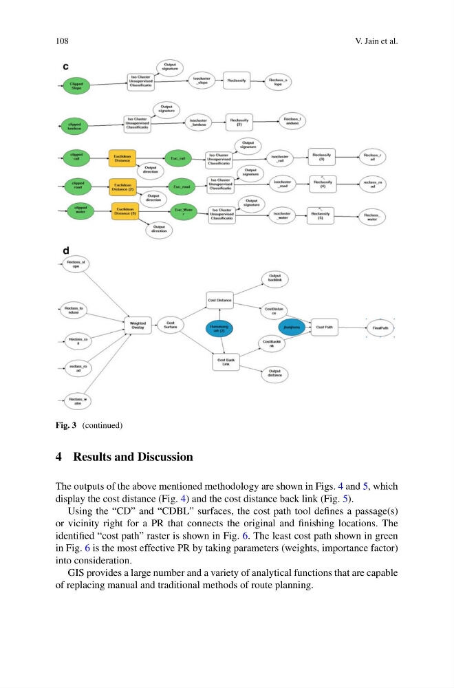
Fig. 3 (continued)
4 Results and Discussion
The outputs of the above mentioned methodology are shown in Figs. 4 and 5, which
display the cost distance (Fig. 4) and the cost distance back link (Fig. 5).
Using the “CD” and “CDBL” surfaces, the cost path tool defines a passage(s)
or vicinity right for a PR that connects the original and finishing locations. The
identified “cost path” raster is shown in Fig. 6. The least cost path shown in green
in Fig. 6 is the most effective PR by taking parameters (weights, importance factor)
into consideration.
GIS provides a large number and a variety of analytical functions that are capable
of replacing manual and traditional methods of route planning.
V. Jain et al.
Fig. 3 (continued)
4 Results and Discussion
The outputs of the above mentioned methodology are shown in Figs. 4 and 5, which
display the cost distance (Fig. 4) and the cost distance back link (Fig. 5).
Using the “CD” and “CDBL” surfaces, the cost path tool defines a passage(s)
or vicinity right for a PR that connects the original and finishing locations. The
identified “cost path” raster is shown in Fig. 6. The least cost path shown in green
in Fig. 6 is the most effective PR by taking parameters (weights, importance factor)
into consideration.
GIS provides a large number and a variety of analytical functions that are capable
of replacing manual and traditional methods of route planning.