

OFDM for Terahertz Wireless Communication Systems
153
6.1 OFDM Signal Distribution
The central limit theorem assumes that the sum of a high number of terms of the
same distribution follows a Gaussian process. Thus, the OFDM signal described by
Eq. (5) can be written for a single OFDM symbol as follows:
Re[x(t)] = x I (t) =
N −1
k=0
I k cos2π
k
N T s
t
(22)
I m[x(t)] = x Q (t) =
N −1
k=0
Q k sin2π
k
N T s
t
(23)
where I k and Q k present the real and imaginary parts of the k-th of c k . The numerical
symbols c k are expected to be statistically i.i.d random variables of zero mean and
variance
P s
2
, where P s is the mean power of the OFDM signal x(t).
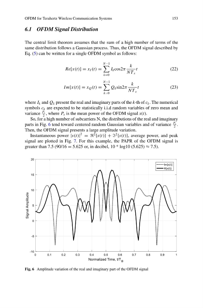
So, for a high number of subcarriers N, the distributions of the real and imaginary
parts in Fig. 6 tend toward centered random Gaussian variables and of variance
P s
2
.
Then, the OFDM signal presents a large amplitude variation.
Instantaneous power |s(t)|
2
= =
2
{s(t)} + +
2
{s(t)}, average power, and peak
signal are plotted in Fig. 7. For this example, the PAPR of the OFDM signal is
greater than 7.5 (90/16 = 5.625 or, in decibel, 10 * log10 (5.625) ≈ 7.5).
Fig. 6 Amplitude variation of the real and imaginary part of the OFDM signal
153
6.1 OFDM Signal Distribution
The central limit theorem assumes that the sum of a high number of terms of the
same distribution follows a Gaussian process. Thus, the OFDM signal described by
Eq. (5) can be written for a single OFDM symbol as follows:
Re[x(t)] = x I (t) =
N −1
k=0
I k cos2π
k
N T s
t
(22)
I m[x(t)] = x Q (t) =
N −1
k=0
Q k sin2π
k
N T s
t
(23)
where I k and Q k present the real and imaginary parts of the k-th of c k . The numerical
symbols c k are expected to be statistically i.i.d random variables of zero mean and
variance
P s
2
, where P s is the mean power of the OFDM signal x(t).
So, for a high number of subcarriers N, the distributions of the real and imaginary
parts in Fig. 6 tend toward centered random Gaussian variables and of variance
P s
2
.
Then, the OFDM signal presents a large amplitude variation.
Instantaneous power |s(t)|
2
= =
2
{s(t)} + +
2
{s(t)}, average power, and peak
signal are plotted in Fig. 7. For this example, the PAPR of the OFDM signal is
greater than 7.5 (90/16 = 5.625 or, in decibel, 10 * log10 (5.625) ≈ 7.5).
Fig. 6 Amplitude variation of the real and imaginary part of the OFDM signal