

150
M. El Ghzaoui and S. Das
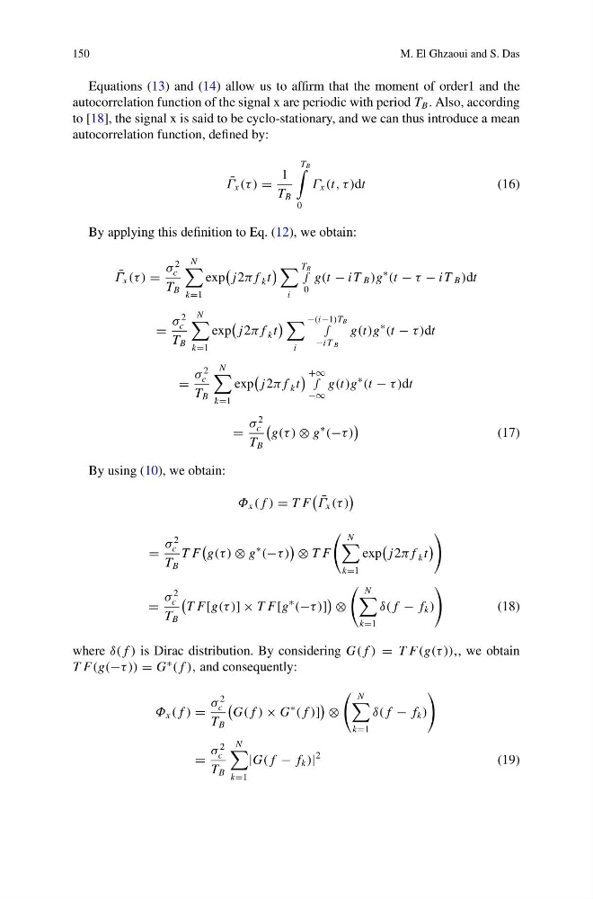
Equations (13) and (14) allow us to affirm that the moment of order1 and the
autocorrelation function of the signal x are periodic with period T B . Also, according
to [18], the signal x is said to be cyclo-stationary, and we can thus introduce a mean
autocorrelation function, defined by:
¯
Γ x (τ ) =
1
T B
T B
0
Γ x (t, τ )dt
(16)
By applying this definition to Eq. (12), we obtain:
¯
Γ x (τ ) =
σ
2
c
T B
N
k=1
exp
j2π f k t
i
T B
∫
0
g(t − i T B )g
∗
(t − τ − i T B )dt
=
σ
2
c
T B
N
k=1
exp
j2π f k t
i
−(i−1)T B
∫
−i T B
g(t)g
∗
(t − τ )dt
=
σ
2
c
T B
N
k=1
exp
j2π f k t
+∞
∫
−∞
g(t)g
∗
(t − τ )dt
=
σ
2
c
T B
g(τ ) ⊗ g
∗
(−τ )
(17)
By using (10), we obtain:
Φ x ( f ) = T F
¯
Γ x (τ )
=
σ
2
c
T B
T F
g(τ ) ⊗ g
∗
(−τ )
⊗ T F
N
k=1
exp
j2π f k t
=
σ
2
c
T B
T F[g(τ )] × T F[g
∗
(−τ )]
⊗
N
k=1
δ( f − f k )
(18)
where δ( f ) is Dirac distribution. By considering G( f ) = T F(g(τ )),, we obtain
T F(g(−τ )) = G
∗
( f ), and consequently:
Φ x ( f ) =
σ
2
c
T B
G( f ) × G
∗
( f )]
⊗
N
k=1
δ( f − f k )
=
σ
2
c
T B
N
k=1
|G( f − f k )|
2
(19)
M. El Ghzaoui and S. Das
Equations (13) and (14) allow us to affirm that the moment of order1 and the
autocorrelation function of the signal x are periodic with period T B . Also, according
to [18], the signal x is said to be cyclo-stationary, and we can thus introduce a mean
autocorrelation function, defined by:
¯
Γ x (τ ) =
1
T B
T B
0
Γ x (t, τ )dt
(16)
By applying this definition to Eq. (12), we obtain:
¯
Γ x (τ ) =
σ
2
c
T B
N
k=1
exp
j2π f k t
i
T B
∫
0
g(t − i T B )g
∗
(t − τ − i T B )dt
=
σ
2
c
T B
N
k=1
exp
j2π f k t
i
−(i−1)T B
∫
−i T B
g(t)g
∗
(t − τ )dt
=
σ
2
c
T B
N
k=1
exp
j2π f k t
+∞
∫
−∞
g(t)g
∗
(t − τ )dt
=
σ
2
c
T B
g(τ ) ⊗ g
∗
(−τ )
(17)
By using (10), we obtain:
Φ x ( f ) = T F
¯
Γ x (τ )
=
σ
2
c
T B
T F
g(τ ) ⊗ g
∗
(−τ )
⊗ T F
N
k=1
exp
j2π f k t
=
σ
2
c
T B
T F[g(τ )] × T F[g
∗
(−τ )]
⊗
N
k=1
δ( f − f k )
(18)
where δ( f ) is Dirac distribution. By considering G( f ) = T F(g(τ )),, we obtain
T F(g(−τ )) = G
∗
( f ), and consequently:
Φ x ( f ) =
σ
2
c
T B
G( f ) × G
∗
( f )]
⊗
N
k=1
δ( f − f k )
=
σ
2
c
T B
N
k=1
|G( f − f k )|
2
(19)