

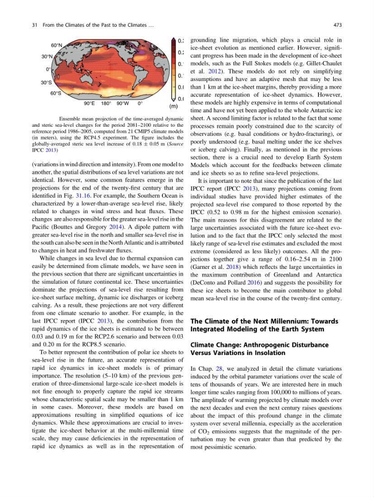
(variations in wind direction and intensity). From one model to
another, the spatial distributions of sea level variations are not
identical. However, some common features emerge in the
projections for the end of the twenty-first century that are
identified in Fig. 31.16. For example, the Southern Ocean is
characterized by a lower-than-average sea-level rise, likely
related to changes in wind stress and heat fluxes. These
changes are also responsible for the greater sea-level rise in the
Pacific (Bouttes and Gregory 2014). A dipole pattern with
greater sea-level rise in the north and smaller sea-level rise in
the south can also be seen in the North Atlantic and is attributed
to changes in heat and freshwater fluxes.
While changes in sea level due to thermal expansion can
easily be determined from climate models, we have seen in
the previous section that there are significant uncertainties in
the simulation of future continental ice. These uncertainties
dominate the projections of sea-level rise resulting from
ice-sheet surface melting, dynamic ice discharges or iceberg
calving. As a result, these projections are not very different
from one climate scenario to another. For example, in the
last IPCC report (IPCC 2013), the contribution from the
rapid dynamics of the ice sheets is estimated to be between
0.03 and 0.19 m for the RCP2.6 scenario and between 0.03
and 0.20 m for the RCP8.5 scenario.
To better represent the contribution of polar ice sheets to
sea-level rise in the future, an accurate representation of
rapid ice dynamics in ice-sheet models is of primary
importance. The resolution (5–10 km) of the previous generation of three-dimensional large-scale ice-sheet models is
not fine enough to properly capture the rapid ice streams
whose characteristic spatial scale may be smaller than 1 km
in some cases. Moreover, these models are based on
approximations resulting in simplified equations of ice
dynamics. While these approximations are crucial to investigate the ice-sheet behavior at the multi-millennial time
scale, they may cause deficiencies in the representation of
rapid ice dynamics as well as in the representation of
grounding line migration, which plays a crucial role in
ice-sheet evolution as mentioned earlier. However, significant progress has been made in the development of ice-sheet
models, such as the Full Stokes models (e.g. Gillet-Chaulet
et al. 2012). These models do not rely on simplifying
assumptions and have an adaptive mesh that may be less
than 1 km at the ice-sheet margins, thereby providing a more
accurate representation of ice-sheet dynamics. However,
these models are highly expensive in terms of computational
time and have not yet been applied to the whole Antarctic ice
sheet. A second limiting factor is related to the fact that some
processes remain poorly constrained due to the scarcity of
observations (e.g. basal conditions or hydro-fracturing), or
poorly understood (e.g. basal melting under the ice shelves
or iceberg calving). Finally, as mentioned in the previous
section, there is a crucial need to develop Earth System
Models which account for the feedbacks between climate
and ice sheets so as to refine sea-level projections.
It is important to note that since the publication of the last
IPCC report (IPCC 2013), many projections coming from
individual studies have provided higher estimates of the
projected sea-level rise compared to those reported by the
IPCC (0.52 to 0.98 m for the highest emission scenario).
The main reasons for this disagreement are related to the
large uncertainties associated with the future ice-sheet evolution and to the fact that the IPCC only selected the most
likely range of sea-level rise estimates and excluded the most
extreme (considered as less likely) outcomes. All the projections together give a range of 0.16–2.54 m in 2100
(Garner et al. 2018) which reflects the large uncertainties in
the maximum contribution of Greenland and Antarctica
(DeConto and Pollard 2016) and suggests the possibility for
these ice sheets to become the main contributor to global
mean sea-level rise in the course of the twenty-first century.
The Climate of the Next Millennium: Towards
Integrated Modeling of the Earth System
Climate Change: Anthropogenic Disturbance
Versus Variations in Insolation
In Chap. 28, we analyzed in detail the climate variations
induced by the orbital parameter variations over the scale of
tens of thousands of years. We are interested here in much
longer time scales ranging from 100,000 to millions of years.
The amplitude of warming projected by climate models over
the next decades and even the next century raises questions
about the impact of this profound change in the climate
system over several millennia, especially as the acceleration
of CO 2 emissions suggests that the magnitude of the perturbation may be even greater than that predicted by the
most pessimistic scenario.
60°S
30°S
0°
30°N
60°N
(m)
0.0
0.0
0.1
0.1
0.2
0.3
90°E 180°
0°
90°W
Fig. 31.16 Ensemble mean projection of the time-averaged dynamic
and steric sea-level changes for the period 2081–2100 relative to the
reference period 1986–2005, computed from 21 CMIP5 climate models
(in meters), using the RCP4.5 experiment. The figure includes the
globally-averaged steric sea level increase of 0.18 ± 0.05 m (Source
IPCC 2013)
31 From the Climates of the Past to the Climates …
473
another, the spatial distributions of sea level variations are not
identical. However, some common features emerge in the
projections for the end of the twenty-first century that are
identified in Fig. 31.16. For example, the Southern Ocean is
characterized by a lower-than-average sea-level rise, likely
related to changes in wind stress and heat fluxes. These
changes are also responsible for the greater sea-level rise in the
Pacific (Bouttes and Gregory 2014). A dipole pattern with
greater sea-level rise in the north and smaller sea-level rise in
the south can also be seen in the North Atlantic and is attributed
to changes in heat and freshwater fluxes.
While changes in sea level due to thermal expansion can
easily be determined from climate models, we have seen in
the previous section that there are significant uncertainties in
the simulation of future continental ice. These uncertainties
dominate the projections of sea-level rise resulting from
ice-sheet surface melting, dynamic ice discharges or iceberg
calving. As a result, these projections are not very different
from one climate scenario to another. For example, in the
last IPCC report (IPCC 2013), the contribution from the
rapid dynamics of the ice sheets is estimated to be between
0.03 and 0.19 m for the RCP2.6 scenario and between 0.03
and 0.20 m for the RCP8.5 scenario.
To better represent the contribution of polar ice sheets to
sea-level rise in the future, an accurate representation of
rapid ice dynamics in ice-sheet models is of primary
importance. The resolution (5–10 km) of the previous generation of three-dimensional large-scale ice-sheet models is
not fine enough to properly capture the rapid ice streams
whose characteristic spatial scale may be smaller than 1 km
in some cases. Moreover, these models are based on
approximations resulting in simplified equations of ice
dynamics. While these approximations are crucial to investigate the ice-sheet behavior at the multi-millennial time
scale, they may cause deficiencies in the representation of
rapid ice dynamics as well as in the representation of
grounding line migration, which plays a crucial role in
ice-sheet evolution as mentioned earlier. However, significant progress has been made in the development of ice-sheet
models, such as the Full Stokes models (e.g. Gillet-Chaulet
et al. 2012). These models do not rely on simplifying
assumptions and have an adaptive mesh that may be less
than 1 km at the ice-sheet margins, thereby providing a more
accurate representation of ice-sheet dynamics. However,
these models are highly expensive in terms of computational
time and have not yet been applied to the whole Antarctic ice
sheet. A second limiting factor is related to the fact that some
processes remain poorly constrained due to the scarcity of
observations (e.g. basal conditions or hydro-fracturing), or
poorly understood (e.g. basal melting under the ice shelves
or iceberg calving). Finally, as mentioned in the previous
section, there is a crucial need to develop Earth System
Models which account for the feedbacks between climate
and ice sheets so as to refine sea-level projections.
It is important to note that since the publication of the last
IPCC report (IPCC 2013), many projections coming from
individual studies have provided higher estimates of the
projected sea-level rise compared to those reported by the
IPCC (0.52 to 0.98 m for the highest emission scenario).
The main reasons for this disagreement are related to the
large uncertainties associated with the future ice-sheet evolution and to the fact that the IPCC only selected the most
likely range of sea-level rise estimates and excluded the most
extreme (considered as less likely) outcomes. All the projections together give a range of 0.16–2.54 m in 2100
(Garner et al. 2018) which reflects the large uncertainties in
the maximum contribution of Greenland and Antarctica
(DeConto and Pollard 2016) and suggests the possibility for
these ice sheets to become the main contributor to global
mean sea-level rise in the course of the twenty-first century.
The Climate of the Next Millennium: Towards
Integrated Modeling of the Earth System
Climate Change: Anthropogenic Disturbance
Versus Variations in Insolation
In Chap. 28, we analyzed in detail the climate variations
induced by the orbital parameter variations over the scale of
tens of thousands of years. We are interested here in much
longer time scales ranging from 100,000 to millions of years.
The amplitude of warming projected by climate models over
the next decades and even the next century raises questions
about the impact of this profound change in the climate
system over several millennia, especially as the acceleration
of CO 2 emissions suggests that the magnitude of the perturbation may be even greater than that predicted by the
most pessimistic scenario.
60°S
30°S
0°
30°N
60°N
(m)
0.0
0.0
0.1
0.1
0.2
0.3
90°E 180°
0°
90°W
Fig. 31.16 Ensemble mean projection of the time-averaged dynamic
and steric sea-level changes for the period 2081–2100 relative to the
reference period 1986–2005, computed from 21 CMIP5 climate models
(in meters), using the RCP4.5 experiment. The figure includes the
globally-averaged steric sea level increase of 0.18 ± 0.05 m (Source
IPCC 2013)
31 From the Climates of the Past to the Climates …
473