

Projecting the Future of the Climate System
Climate Response to a Doubling of CO 2 : Forcings
and Feedbacks
Perturbations that modify the energy balance of the climate
system are quantified in terms of energy flux at the top of the
atmosphere. Quantifying the forcing due to a variation in
average insolation is immediate. For a change in the
greenhouse gas concentration, a radiative model is used to
calculate how these changes affect fluxes at the top of the
atmosphere. Since the late 1980s, it is now possible to perform these calculations using radiative transfer codes and
spectral databases, provided that all other atmospheric (e.g.
clouds, aerosols) and surface (e.g. snow cover) characteristics are assumed to be fixed. For a doubling of the atmospheric CO 2 concentration, the global mean annual radiative
forcing at the top of the atmosphere is 3.7 ± 0.2 W/m
2 . As
we focus on slow climate variations, the calculation of the
radiative forcing takes into account the rapid adjustment of
the stratospheric temperature.
In response to the radiative forcing DQ, the different
climate models simulate a temperature change at equilibrium
DT which is different from one model to another. These
differences are difficult to analyze and interpret directly
because of the high level of model complexity. A standard
method to identify the origin of these differences is the
feedback analysis (see, for example, Dufresne and Saint-Lu
2016). From the temperature change at equilibrium DT, a
‘feedback parameter’ k is defined:
k ¼ ÀDQ=DT:
By writing this equation in the form k  DT +DQ = 0,
we see that k  DT represents the variation in the average
flux at the top of the atmosphere necessary to compensate for
the radiative forcing DQ. We can therefore write k = −dF/
dT, with F being the net radiative flux at the top of the
atmosphere, counted as positive when it is descending. This
derivative can be decomposed, in the first order, as a sum of
partial derivatives:
k ¼ ÀR@F=@X Â @X=@T
The sum over X is the sum of all the X variables affecting
the radiative balance at the top of the atmosphere and that are
modified when the surface temperature changes. These are
mainly the three-dimensional fields of temperature, water
vapor and clouds, and the two-dimensional fields of surface
albedo. The change in the temperature field is generally
broken down into two terms, one corresponding to a uniform
temperature change, the other to the non-uniform part of the
temperature change. Finally, the parameter k can be
decomposed as follows:
k ¼ k P þ k L þ k c þ k w þ k a
The terms of the right-hand side are the respective feedback
parameters: Planck k P (uniform temperature change), the
temperature gradient k L (non-uniform part of the temperature
change), clouds k c , water vapor k w and surface albedo k a .
These parameters are often calculated as follows using the
partial radiative perturbation method. For a given climate
model, two simulations are carried out, a reference one and a
perturbed one. The fluxes at the top of the atmosphere are
calculated off-line from the outputs of the reference simulation using a radiative code. They are then recalculated by
replacing the values of some variables (temperature,
humidity, clouds, surface albedo) from the reference simulation with the corresponding values from the perturbed
simulation. The difference between these two fluxes gives
the sensitivity of the fluxes at the top of the atmosphere to a
perturbation of each of the variables.
The particular Planck parameter k P corresponds to the
response of the flux at the top of the atmosphere to a uniform
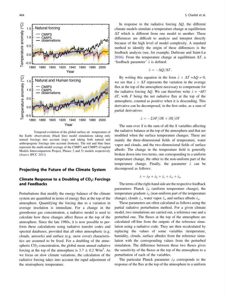
Fig. 31.9 Temporal evolution of the global surface air temperature of
the Earth: observations (black line) model simulations taking only
natural forcings into account (top), and taking both natural and
anthropogenic forcings into account (bottom). The red and blue lines
represent the multi-model average of the CMIP3 and CMIP5 (Coupled
Models Intercomparison Project, Phases 3 and 5) models respectively
(Source IPCC 2013)
464
S. Charbit et al.
Climate Response to a Doubling of CO 2 : Forcings
and Feedbacks
Perturbations that modify the energy balance of the climate
system are quantified in terms of energy flux at the top of the
atmosphere. Quantifying the forcing due to a variation in
average insolation is immediate. For a change in the
greenhouse gas concentration, a radiative model is used to
calculate how these changes affect fluxes at the top of the
atmosphere. Since the late 1980s, it is now possible to perform these calculations using radiative transfer codes and
spectral databases, provided that all other atmospheric (e.g.
clouds, aerosols) and surface (e.g. snow cover) characteristics are assumed to be fixed. For a doubling of the atmospheric CO 2 concentration, the global mean annual radiative
forcing at the top of the atmosphere is 3.7 ± 0.2 W/m
2 . As
we focus on slow climate variations, the calculation of the
radiative forcing takes into account the rapid adjustment of
the stratospheric temperature.
In response to the radiative forcing DQ, the different
climate models simulate a temperature change at equilibrium
DT which is different from one model to another. These
differences are difficult to analyze and interpret directly
because of the high level of model complexity. A standard
method to identify the origin of these differences is the
feedback analysis (see, for example, Dufresne and Saint-Lu
2016). From the temperature change at equilibrium DT, a
‘feedback parameter’ k is defined:
k ¼ ÀDQ=DT:
By writing this equation in the form k  DT +DQ = 0,
we see that k  DT represents the variation in the average
flux at the top of the atmosphere necessary to compensate for
the radiative forcing DQ. We can therefore write k = −dF/
dT, with F being the net radiative flux at the top of the
atmosphere, counted as positive when it is descending. This
derivative can be decomposed, in the first order, as a sum of
partial derivatives:
k ¼ ÀR@F=@X Â @X=@T
The sum over X is the sum of all the X variables affecting
the radiative balance at the top of the atmosphere and that are
modified when the surface temperature changes. These are
mainly the three-dimensional fields of temperature, water
vapor and clouds, and the two-dimensional fields of surface
albedo. The change in the temperature field is generally
broken down into two terms, one corresponding to a uniform
temperature change, the other to the non-uniform part of the
temperature change. Finally, the parameter k can be
decomposed as follows:
k ¼ k P þ k L þ k c þ k w þ k a
The terms of the right-hand side are the respective feedback
parameters: Planck k P (uniform temperature change), the
temperature gradient k L (non-uniform part of the temperature
change), clouds k c , water vapor k w and surface albedo k a .
These parameters are often calculated as follows using the
partial radiative perturbation method. For a given climate
model, two simulations are carried out, a reference one and a
perturbed one. The fluxes at the top of the atmosphere are
calculated off-line from the outputs of the reference simulation using a radiative code. They are then recalculated by
replacing the values of some variables (temperature,
humidity, clouds, surface albedo) from the reference simulation with the corresponding values from the perturbed
simulation. The difference between these two fluxes gives
the sensitivity of the fluxes at the top of the atmosphere to a
perturbation of each of the variables.
The particular Planck parameter k P corresponds to the
response of the flux at the top of the atmosphere to a uniform
Fig. 31.9 Temporal evolution of the global surface air temperature of
the Earth: observations (black line) model simulations taking only
natural forcings into account (top), and taking both natural and
anthropogenic forcings into account (bottom). The red and blue lines
represent the multi-model average of the CMIP3 and CMIP5 (Coupled
Models Intercomparison Project, Phases 3 and 5) models respectively
(Source IPCC 2013)
464
S. Charbit et al.