

incoming solar radiation), and is higher over continental
areas than above the oceans, mainly because of the lower
thermal inertia of the continents.
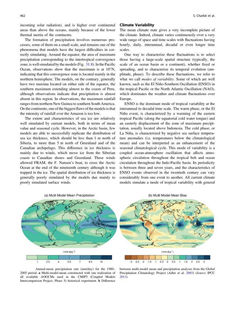
The formation of precipitation involves numerous processes, some of them on a small scale, and remains one of the
phenomena that models have the largest difficulties in correctly simulating. Around the equator, the area of maximum
precipitation corresponding to the intertropical convergence
zone, is well simulated by the models (Fig. 31.8). In the Pacific
Ocean, observations show that the maximum is at 10°N,
indicating that this convergence zone is located mainly in the
northern hemisphere. The models, on the contrary, generally
have two maxima located on either side of the equator, the
southern maximum extending almost to the coasts of Peru,
although observations indicate that precipitation is almost
absent in this region. In observations, the maximum rainfall
ranges from northern New Guinea to southern South America.
On the continents, one of the biggest flaws of the models is that
the intensity of rainfall over the Amazon is too low.
The extent and characteristics of sea ice are relatively
well simulated by current models, both in terms of mean
value and seasonal cycle. However, in the Arctic basin, few
models are able to successfully replicate the distribution of
sea ice thickness, which should be less than 1 m north of
Siberia, to more than 5 m north of Greenland and of the
Canadian archipelago. This difference in ice thickness is
mainly due to winds, which move ice from the Siberian
coasts to Canadian shores and Greenland. These winds
allowed FRAM, the F. Nansen’s boat, to cross the Arctic
Ocean at the end of the nineteenth century although it was
trapped in the ice. The spatial distribution of ice thickness is
generally poorly simulated by the models due mainly to
poorly simulated surface winds.
Climate Variability
The mean climate state gives a very incomplete picture of
the climate. Indeed, climate varies continuously over a very
wide range of space and time scales with fluctuations having
hourly, daily, interannual, decadal or even longer time
scales.
One way to characterize these fluctuations is to select
those having a large-scale spatial structure (typically, the
scale of an ocean basin or a continent), whether fixed or
spreading, and to characterize its temporal evolution (amplitude, phase). To describe these fluctuations, we refer to
what we call modes of variability. Some of which are well
known, such as the El Niño-Southern Oscillation (ENSO) in
the tropical Pacific or the North Atlantic Oscillation (NAO),
which dominates the weather and climate fluctuations over
Europe.
ENSO is the dominant mode of tropical variability at the
interannual to decadal time scale. The warm phase, or the El
Niño event, is characterized by a warming of the eastern
tropical Pacific (along the equatorial cold water tongue) and
an easterly displacement of the zone of maximum precipitation, usually located above Indonesia. The cold phase, or
La Niña, is characterized by negative sea surface temperature anomalies (i.e. temperatures below the climatological
mean) and can be interpreted as an enhancement of the
seasonal climatological cycle. This mode of variability is a
coupled ocean-atmosphere oscillation that affects atmospheric circulation throughout the tropical belt and ocean
circulation throughout the Indo-Pacific basin. Its periodicity
is between three and seven years, and the characteristics of
ENSO events observed in the twentieth century can vary
considerably from one event to another. All current climate
models simulate a mode of tropical variability with general
Fig. 31.8 Annual-mean precipitation rate (mm/day) for the 1980–
2005 period. a Multi-model-mean constructed with one realization of
all available AOGCMs used in the CMIP5 (Coupled Models
Intercomparison Project, Phase 5) historical experiment. b Difference
between multi-model mean and precipitation analyses from the Global
Precipitation Climatology Project (Adler et al. 2003) (Source IPCC
2013)
462
S. Charbit et al.
areas than above the oceans, mainly because of the lower
thermal inertia of the continents.
The formation of precipitation involves numerous processes, some of them on a small scale, and remains one of the
phenomena that models have the largest difficulties in correctly simulating. Around the equator, the area of maximum
precipitation corresponding to the intertropical convergence
zone, is well simulated by the models (Fig. 31.8). In the Pacific
Ocean, observations show that the maximum is at 10°N,
indicating that this convergence zone is located mainly in the
northern hemisphere. The models, on the contrary, generally
have two maxima located on either side of the equator, the
southern maximum extending almost to the coasts of Peru,
although observations indicate that precipitation is almost
absent in this region. In observations, the maximum rainfall
ranges from northern New Guinea to southern South America.
On the continents, one of the biggest flaws of the models is that
the intensity of rainfall over the Amazon is too low.
The extent and characteristics of sea ice are relatively
well simulated by current models, both in terms of mean
value and seasonal cycle. However, in the Arctic basin, few
models are able to successfully replicate the distribution of
sea ice thickness, which should be less than 1 m north of
Siberia, to more than 5 m north of Greenland and of the
Canadian archipelago. This difference in ice thickness is
mainly due to winds, which move ice from the Siberian
coasts to Canadian shores and Greenland. These winds
allowed FRAM, the F. Nansen’s boat, to cross the Arctic
Ocean at the end of the nineteenth century although it was
trapped in the ice. The spatial distribution of ice thickness is
generally poorly simulated by the models due mainly to
poorly simulated surface winds.
Climate Variability
The mean climate state gives a very incomplete picture of
the climate. Indeed, climate varies continuously over a very
wide range of space and time scales with fluctuations having
hourly, daily, interannual, decadal or even longer time
scales.
One way to characterize these fluctuations is to select
those having a large-scale spatial structure (typically, the
scale of an ocean basin or a continent), whether fixed or
spreading, and to characterize its temporal evolution (amplitude, phase). To describe these fluctuations, we refer to
what we call modes of variability. Some of which are well
known, such as the El Niño-Southern Oscillation (ENSO) in
the tropical Pacific or the North Atlantic Oscillation (NAO),
which dominates the weather and climate fluctuations over
Europe.
ENSO is the dominant mode of tropical variability at the
interannual to decadal time scale. The warm phase, or the El
Niño event, is characterized by a warming of the eastern
tropical Pacific (along the equatorial cold water tongue) and
an easterly displacement of the zone of maximum precipitation, usually located above Indonesia. The cold phase, or
La Niña, is characterized by negative sea surface temperature anomalies (i.e. temperatures below the climatological
mean) and can be interpreted as an enhancement of the
seasonal climatological cycle. This mode of variability is a
coupled ocean-atmosphere oscillation that affects atmospheric circulation throughout the tropical belt and ocean
circulation throughout the Indo-Pacific basin. Its periodicity
is between three and seven years, and the characteristics of
ENSO events observed in the twentieth century can vary
considerably from one event to another. All current climate
models simulate a mode of tropical variability with general
Fig. 31.8 Annual-mean precipitation rate (mm/day) for the 1980–
2005 period. a Multi-model-mean constructed with one realization of
all available AOGCMs used in the CMIP5 (Coupled Models
Intercomparison Project, Phase 5) historical experiment. b Difference
between multi-model mean and precipitation analyses from the Global
Precipitation Climatology Project (Adler et al. 2003) (Source IPCC
2013)
462
S. Charbit et al.