

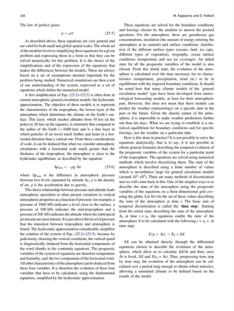
The law of perfect gases:
p ¼ qrt
ð25:5Þ
As described above, these equations are very general and
are valid for both small and global spatial scales. The whole art
of the modeler involves simplifying these equations for a given
problem and expressing them in a form so that they can be
solved numerically for this problem. It is the choice of the
simplifications and of the expression of the equations that
makes the differences between the models. These are always
based on a set of assumptions deemed important for the
problem being studied. Numerical simulations are then a test
of our understanding of the system, expressed as a set of
equations which define the numerical model.
A first simplification of Eqs. (25.2)–(25.5) is often done in
current atmospheric general circulation models: the hydrostatic
approximation. The objective of these models is to represent
the characteristics of the troposphere, the lowest layer of the
atmosphere which determines the climate on the Earth’s surface. This layer, which reaches altitudes from 10 km (at the
poles) to 20 km (at the equator), is extremely thin compared to
the radius of the Earth (*6400 km) and is a fine layer in
which particles of air travel much further and faster in a horizontal direction than a vertical one. From these considerations
of scale, it can be deduced that when we consider atmospheric
circulations with a horizontal scale much greater than the
thickness of the troposphere, the atmosphere is close to the
hydrostatic equilibrium, as described by the equation:
Dp atm ¼ Àqg Dz
ð25:6Þ
where Dp atm is the difference in atmospheric pressure
between two levels separated by altitude Dz, q is the density
of air, g is the acceleration due to gravity.
This direct relationship between pressure and altitude leads
atmospheric specialists to often present variations in vertical
atmospheric properties as a function of pressure: for example, a
pressure of 1000 hPa indicates a level close to the surface, a
pressure of 500 hPa indicates the mid-troposphere and a
pressure of 200 hPa indicates the altitude where the subtropical
jet streams are most intense. It is just above this level of pressure
that the transition between troposphere and stratosphere is
found. The hydrostatic approximation considerably simplifies
the solution of the system of Eqs. (25.2)–(25.5), because by
judiciously choosing the vertical coordinate, the vertical speed
is diagnostically deduced from the horizontal components of
the wind (thanks to the continuity equation). The prognostic
variables of the system of equations are therefore temperature
and humidity, and the two components of the horizontal wind.
All other characteristics of the atmosphere can be deduced from
these four variables. It is therefore the evolution of these four
variables that have to be calculated, using the fundamental
equations, simplified by the hydrostatic approximation.
These equations are solved for the boundary conditions
and forcings chosen by the modeler to answer the posited
questions. For the atmosphere, these are greenhouse gas
concentrations, insolation (the amount of energy entering the
atmosphere at its summit) and surface conditions: distribution of the different surface types (oceans, land, ice caps,
different types of vegetation), orography, ocean surface
conditions (temperature and sea ice coverage). An initial
state for all the prognostic variables of the model is also
chosen. From this initial state, the evolution of the atmosphere is calculated over the time necessary for its characteristics (temperature, precipitation, wind etc.) to be in
equilibrium with the imposed boundary conditions. It should
be noted here that many climate models of the ‘general
circulation model’ type have been developed from meteorological forecasting models, at least for their atmospheric
part. However, this does not mean that these models can
predict the weather (meteorology) on a specific date in the
past or the future. Given the chaotic nature of the atmosphere, it is impossible to make weather predictions further
out than ten days. What we are trying to establish is a statistical equilibrium for boundary conditions and for specific
forcings, not the weather on a particular date.
How is this done in practice? It is not possible to solve the
equations analytically, that is to say, it is not possible to
obtain general formulae describing the temporal evolution of
the prognostic variables of the system for a particular point
of the troposphere. The equations are solved using numerical
methods which involve discretizing them. The state of the
atmosphere is described using a finite number of values
which is nevertheless large for general circulation models
(around 10
5
–10
6 ). There are many methods of discretization
and we will come back to this. One of the simplest ways is to
describe the state of the atmosphere using the prognostic
variables of the equations on a three-dimensional grid covering the globe. Let X(t) be the set of these values describing
the state of the atmosphere at time t. The basic unit of
temporal discretization is called the ‘time step’. Starting
from the initial state, describing the state of the atmosphere
X 0 at time t = t 0 , the equations enable the state of the
atmosphere X to be calculated with the following t = t 0 + Dt
time step:
X t 0 þ Dt
ð
Þ ¼X 0 þ DX
DX can be obtained directly through the differential
equations chosen to describe the evolution of the atmosphere, which allow us to calculate DX/Dt and then, once
Dt is fixed, DX and X(t 0 + Dt). Thus, progressing time step
by time step, the evolution of the atmosphere can be calculated over a period long enough to obtain robust statistics,
allowing a simulated climate to be defined based on the
results of the model.
326
M. Kageyama and D. Paillard
p ¼ qrt
ð25:5Þ
As described above, these equations are very general and
are valid for both small and global spatial scales. The whole art
of the modeler involves simplifying these equations for a given
problem and expressing them in a form so that they can be
solved numerically for this problem. It is the choice of the
simplifications and of the expression of the equations that
makes the differences between the models. These are always
based on a set of assumptions deemed important for the
problem being studied. Numerical simulations are then a test
of our understanding of the system, expressed as a set of
equations which define the numerical model.
A first simplification of Eqs. (25.2)–(25.5) is often done in
current atmospheric general circulation models: the hydrostatic
approximation. The objective of these models is to represent
the characteristics of the troposphere, the lowest layer of the
atmosphere which determines the climate on the Earth’s surface. This layer, which reaches altitudes from 10 km (at the
poles) to 20 km (at the equator), is extremely thin compared to
the radius of the Earth (*6400 km) and is a fine layer in
which particles of air travel much further and faster in a horizontal direction than a vertical one. From these considerations
of scale, it can be deduced that when we consider atmospheric
circulations with a horizontal scale much greater than the
thickness of the troposphere, the atmosphere is close to the
hydrostatic equilibrium, as described by the equation:
Dp atm ¼ Àqg Dz
ð25:6Þ
where Dp atm is the difference in atmospheric pressure
between two levels separated by altitude Dz, q is the density
of air, g is the acceleration due to gravity.
This direct relationship between pressure and altitude leads
atmospheric specialists to often present variations in vertical
atmospheric properties as a function of pressure: for example, a
pressure of 1000 hPa indicates a level close to the surface, a
pressure of 500 hPa indicates the mid-troposphere and a
pressure of 200 hPa indicates the altitude where the subtropical
jet streams are most intense. It is just above this level of pressure
that the transition between troposphere and stratosphere is
found. The hydrostatic approximation considerably simplifies
the solution of the system of Eqs. (25.2)–(25.5), because by
judiciously choosing the vertical coordinate, the vertical speed
is diagnostically deduced from the horizontal components of
the wind (thanks to the continuity equation). The prognostic
variables of the system of equations are therefore temperature
and humidity, and the two components of the horizontal wind.
All other characteristics of the atmosphere can be deduced from
these four variables. It is therefore the evolution of these four
variables that have to be calculated, using the fundamental
equations, simplified by the hydrostatic approximation.
These equations are solved for the boundary conditions
and forcings chosen by the modeler to answer the posited
questions. For the atmosphere, these are greenhouse gas
concentrations, insolation (the amount of energy entering the
atmosphere at its summit) and surface conditions: distribution of the different surface types (oceans, land, ice caps,
different types of vegetation), orography, ocean surface
conditions (temperature and sea ice coverage). An initial
state for all the prognostic variables of the model is also
chosen. From this initial state, the evolution of the atmosphere is calculated over the time necessary for its characteristics (temperature, precipitation, wind etc.) to be in
equilibrium with the imposed boundary conditions. It should
be noted here that many climate models of the ‘general
circulation model’ type have been developed from meteorological forecasting models, at least for their atmospheric
part. However, this does not mean that these models can
predict the weather (meteorology) on a specific date in the
past or the future. Given the chaotic nature of the atmosphere, it is impossible to make weather predictions further
out than ten days. What we are trying to establish is a statistical equilibrium for boundary conditions and for specific
forcings, not the weather on a particular date.
How is this done in practice? It is not possible to solve the
equations analytically, that is to say, it is not possible to
obtain general formulae describing the temporal evolution of
the prognostic variables of the system for a particular point
of the troposphere. The equations are solved using numerical
methods which involve discretizing them. The state of the
atmosphere is described using a finite number of values
which is nevertheless large for general circulation models
(around 10
5
–10
6 ). There are many methods of discretization
and we will come back to this. One of the simplest ways is to
describe the state of the atmosphere using the prognostic
variables of the equations on a three-dimensional grid covering the globe. Let X(t) be the set of these values describing
the state of the atmosphere at time t. The basic unit of
temporal discretization is called the ‘time step’. Starting
from the initial state, describing the state of the atmosphere
X 0 at time t = t 0 , the equations enable the state of the
atmosphere X to be calculated with the following t = t 0 + Dt
time step:
X t 0 þ Dt
ð
Þ ¼X 0 þ DX
DX can be obtained directly through the differential
equations chosen to describe the evolution of the atmosphere, which allow us to calculate DX/Dt and then, once
Dt is fixed, DX and X(t 0 + Dt). Thus, progressing time step
by time step, the evolution of the atmosphere can be calculated over a period long enough to obtain robust statistics,
allowing a simulated climate to be defined based on the
results of the model.
326
M. Kageyama and D. Paillard