

system. We can therefore focus on the asymptotic behavior
alone in the model, that is to say its behavior from moment t 1
onwards, after this initial condition is forgotten. Conversely,
the transitional phase between the beginning of the simulation at t 0 and time t 1 , is highly dependent on the initial
condition selected, and the results will only be relevant if
this condition is correctly understood. Knowing that the
duration t 1 − t 0 is a few weeks for atmospheric dynamics,
we see here an essential difference between a climate model
and a meteorological model. For the latter, this transitory
phase is the most interesting. A major difficulty in weather
forecasting is to provide, in real time, an initial condition that
represents the state of the atmosphere ‘now’ in order to be
able to anticipate its state in the hours and days to come. For
the climatologist, the initial state of the atmosphere is of little
importance, since it will be quickly forgotten. It should be
noted, however, that this may not be the case for the initial
state of other physical components of the system, such as the
ocean, which have much longer time constants.
Nevertheless, this initial state of the atmosphere is not
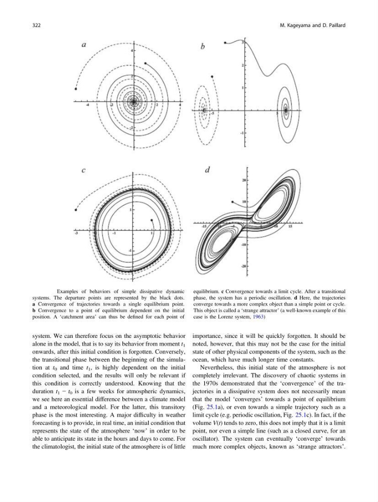
completely irrelevant. The discovery of chaotic systems in
the 1970s demonstrated that the ‘convergence’ of the trajectories in a dissipative system does not necessarily mean
that the model ‘converges’ towards a point of equilibrium
(Fig. 25.1a), or even towards a simple trajectory such as a
limit cycle (e.g. periodic oscillation, Fig. 25.1c). In fact, if the
volume V(t) tends to zero, this does not imply that it is a limit
point, nor even a simple line (such as a closed curve, for an
oscillator). The system can eventually ‘converge’ towards
much more complex objects, known as ‘strange attractors’.
Fig. 25.1 Examples of behaviors of simple dissipative dynamic
systems. The departure points are represented by the black dots.
a Convergence of trajectories towards a single equilibrium point.
b Convergence to a point of equilibrium dependent on the initial
position. A ‘catchment area’ can thus be defined for each point of
equilibrium. c Convergence towards a limit cycle. After a transitional
phase, the system has a periodic oscillation. d Here, the trajectories
converge towards a more complex object than a simple point or cycle.
This object is called a ‘strange attractor’ (a well-known example of this
case is the Lorenz system, 1963)
322
M. Kageyama and D. Paillard
alone in the model, that is to say its behavior from moment t 1
onwards, after this initial condition is forgotten. Conversely,
the transitional phase between the beginning of the simulation at t 0 and time t 1 , is highly dependent on the initial
condition selected, and the results will only be relevant if
this condition is correctly understood. Knowing that the
duration t 1 − t 0 is a few weeks for atmospheric dynamics,
we see here an essential difference between a climate model
and a meteorological model. For the latter, this transitory
phase is the most interesting. A major difficulty in weather
forecasting is to provide, in real time, an initial condition that
represents the state of the atmosphere ‘now’ in order to be
able to anticipate its state in the hours and days to come. For
the climatologist, the initial state of the atmosphere is of little
importance, since it will be quickly forgotten. It should be
noted, however, that this may not be the case for the initial
state of other physical components of the system, such as the
ocean, which have much longer time constants.
Nevertheless, this initial state of the atmosphere is not
completely irrelevant. The discovery of chaotic systems in
the 1970s demonstrated that the ‘convergence’ of the trajectories in a dissipative system does not necessarily mean
that the model ‘converges’ towards a point of equilibrium
(Fig. 25.1a), or even towards a simple trajectory such as a
limit cycle (e.g. periodic oscillation, Fig. 25.1c). In fact, if the
volume V(t) tends to zero, this does not imply that it is a limit
point, nor even a simple line (such as a closed curve, for an
oscillator). The system can eventually ‘converge’ towards
much more complex objects, known as ‘strange attractors’.
Fig. 25.1 Examples of behaviors of simple dissipative dynamic
systems. The departure points are represented by the black dots.
a Convergence of trajectories towards a single equilibrium point.
b Convergence to a point of equilibrium dependent on the initial
position. A ‘catchment area’ can thus be defined for each point of
equilibrium. c Convergence towards a limit cycle. After a transitional
phase, the system has a periodic oscillation. d Here, the trajectories
converge towards a more complex object than a simple point or cycle.
This object is called a ‘strange attractor’ (a well-known example of this
case is the Lorenz system, 1963)
322
M. Kageyama and D. Paillard