

resulting in more carbon in the ocean when the AABW
occupies relatively more volume than the NADW (Brovkin
et al. 2012). This is referred to as the “standing volume
effect” (Skinner 2009).
Changes of ocean circulation could be due to changes of
winds (Anderson et al. 2009; Toggweiler et al. 2006). But
data show no clear evidence of large wind changes (Kohfeld
et al. 2013) and model simulations have shown that this is
unlikely to have had a strong effect on the carbon cycle
(Menviel et al. 2008a). It could also be linked to ocean
diffusion (Bouttes et al. 2009, 2011) and particularly to
bottom topography induced diffusion (De Boer and Hogg
2014). Alternatively, it could be linked to sea ice changes
and modifications in bottom water formation (Ferrari et al.
2014; Bouttes et al. 2010). Indeed, sea ice formation around
Antarctica was probably enhanced, especially during winter
(Gersonde et al. 2005). Yet models usually fail to represent
glacial sea ice extent (Roche et al. 2012; Goosse et al. 2013;
Marzocchi and Jansen 2017). Improving sea ice formation in
models during the LGM and the sinking of dense water
around Antarctica should help towards explaining the glacial
atmospheric CO 2 concentration.
Finally, on longer timescales of a few thousand years,
carbonate compensation amplifies the increase of oceanic
carbon storage, by maintaining a balance between inputs and
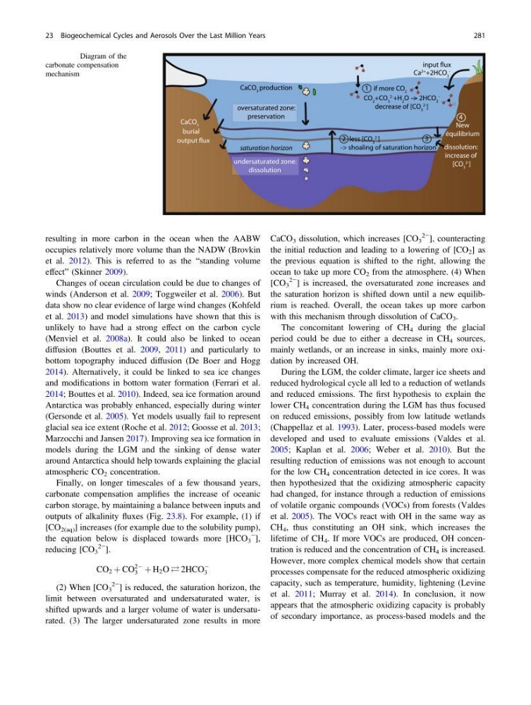
outputs of alkalinity fluxes (Fig. 23.8). For example, (1) if
[CO 2(aq) ] increases (for example due to the solubility pump),
the equation below is displaced towards more [HCO 3
− ],
reducing [CO 3
2− ].
CO 2 þ CO
2À
3 þ H 2 O 2HCO
À
3
(2) When [CO 3
2− ] is reduced, the saturation horizon, the
limit between oversaturated and undersaturated water, is
shifted upwards and a larger volume of water is undersaturated. (3) The larger undersaturated zone results in more
CaCO 3 dissolution, which increases [CO 3
2− ], counteracting
the initial reduction and leading to a lowering of [CO 2 ] as
the previous equation is shifted to the right, allowing the
ocean to take up more CO 2 from the atmosphere. (4) When
[CO 3
2− ] is increased, the oversaturated zone increases and
the saturation horizon is shifted down until a new equilibrium is reached. Overall, the ocean takes up more carbon
with this mechanism through dissolution of CaCO 3 .
The concomitant lowering of CH 4 during the glacial
period could be due to either a decrease in CH 4 sources,
mainly wetlands, or an increase in sinks, mainly more oxidation by increased OH.
During the LGM, the colder climate, larger ice sheets and
reduced hydrological cycle all led to a reduction of wetlands
and reduced emissions. The first hypothesis to explain the
lower CH 4 concentration during the LGM has thus focused
on reduced emissions, possibly from low latitude wetlands
(Chappellaz et al. 1993). Later, process-based models were
developed and used to evaluate emissions (Valdes et al.
2005; Kaplan et al. 2006; Weber et al. 2010). But the
resulting reduction of emissions was not enough to account
for the low CH 4 concentration detected in ice cores. It was
then hypothesized that the oxidizing atmospheric capacity
had changed, for instance through a reduction of emissions
of volatile organic compounds (VOCs) from forests (Valdes
et al. 2005). The VOCs react with OH in the same way as
CH 4 , thus constituting an OH sink, which increases the
lifetime of CH 4 . If more VOCs are produced, OH concentration is reduced and the concentration of CH 4 is increased.
However, more complex chemical models show that certain
processes compensate for the reduced atmospheric oxidizing
capacity, such as temperature, humidity, lightening (Levine
et al. 2011; Murray et al. 2014). In conclusion, it now
appears that the atmospheric oxidizing capacity is probably
of secondary importance, as process-based models and the
Ca
2+
+2HCO 3
-
less [CO 3
2- ]
-> shoaling of saturation horizon
CO 2 +CO 3
2- +H 2 O > 2HCO 3
-
decrease of [CO 3
2]
dissolution:
increase of
[CO 3
2- ]
New
équilibrium
1
2
3
4
CaCO 3
if more CO 2
burial
output flux
input flux
saturation horizon
CaCO 3 production
oversaturated zone:
preservation
undersaturated zone:
dissolution
Fig. 23.8 Diagram of the
carbonate compensation
mechanism
23 Biogeochemical Cycles and Aerosols Over the Last Million Years
281
occupies relatively more volume than the NADW (Brovkin
et al. 2012). This is referred to as the “standing volume
effect” (Skinner 2009).
Changes of ocean circulation could be due to changes of
winds (Anderson et al. 2009; Toggweiler et al. 2006). But
data show no clear evidence of large wind changes (Kohfeld
et al. 2013) and model simulations have shown that this is
unlikely to have had a strong effect on the carbon cycle
(Menviel et al. 2008a). It could also be linked to ocean
diffusion (Bouttes et al. 2009, 2011) and particularly to
bottom topography induced diffusion (De Boer and Hogg
2014). Alternatively, it could be linked to sea ice changes
and modifications in bottom water formation (Ferrari et al.
2014; Bouttes et al. 2010). Indeed, sea ice formation around
Antarctica was probably enhanced, especially during winter
(Gersonde et al. 2005). Yet models usually fail to represent
glacial sea ice extent (Roche et al. 2012; Goosse et al. 2013;
Marzocchi and Jansen 2017). Improving sea ice formation in
models during the LGM and the sinking of dense water
around Antarctica should help towards explaining the glacial
atmospheric CO 2 concentration.
Finally, on longer timescales of a few thousand years,
carbonate compensation amplifies the increase of oceanic
carbon storage, by maintaining a balance between inputs and
outputs of alkalinity fluxes (Fig. 23.8). For example, (1) if
[CO 2(aq) ] increases (for example due to the solubility pump),
the equation below is displaced towards more [HCO 3
− ],
reducing [CO 3
2− ].
CO 2 þ CO
2À
3 þ H 2 O 2HCO
À
3
(2) When [CO 3
2− ] is reduced, the saturation horizon, the
limit between oversaturated and undersaturated water, is
shifted upwards and a larger volume of water is undersaturated. (3) The larger undersaturated zone results in more
CaCO 3 dissolution, which increases [CO 3
2− ], counteracting
the initial reduction and leading to a lowering of [CO 2 ] as
the previous equation is shifted to the right, allowing the
ocean to take up more CO 2 from the atmosphere. (4) When
[CO 3
2− ] is increased, the oversaturated zone increases and
the saturation horizon is shifted down until a new equilibrium is reached. Overall, the ocean takes up more carbon
with this mechanism through dissolution of CaCO 3 .
The concomitant lowering of CH 4 during the glacial
period could be due to either a decrease in CH 4 sources,
mainly wetlands, or an increase in sinks, mainly more oxidation by increased OH.
During the LGM, the colder climate, larger ice sheets and
reduced hydrological cycle all led to a reduction of wetlands
and reduced emissions. The first hypothesis to explain the
lower CH 4 concentration during the LGM has thus focused
on reduced emissions, possibly from low latitude wetlands
(Chappellaz et al. 1993). Later, process-based models were
developed and used to evaluate emissions (Valdes et al.
2005; Kaplan et al. 2006; Weber et al. 2010). But the
resulting reduction of emissions was not enough to account
for the low CH 4 concentration detected in ice cores. It was
then hypothesized that the oxidizing atmospheric capacity
had changed, for instance through a reduction of emissions
of volatile organic compounds (VOCs) from forests (Valdes
et al. 2005). The VOCs react with OH in the same way as
CH 4 , thus constituting an OH sink, which increases the
lifetime of CH 4 . If more VOCs are produced, OH concentration is reduced and the concentration of CH 4 is increased.
However, more complex chemical models show that certain
processes compensate for the reduced atmospheric oxidizing
capacity, such as temperature, humidity, lightening (Levine
et al. 2011; Murray et al. 2014). In conclusion, it now
appears that the atmospheric oxidizing capacity is probably
of secondary importance, as process-based models and the
Ca
2+
+2HCO 3
-
less [CO 3
2- ]
-> shoaling of saturation horizon
CO 2 +CO 3
2- +H 2 O > 2HCO 3
-
decrease of [CO 3
2]
dissolution:
increase of
[CO 3
2- ]
New
équilibrium
1
2
3
4
CaCO 3
if more CO 2
burial
output flux
input flux
saturation horizon
CaCO 3 production
oversaturated zone:
preservation
undersaturated zone:
dissolution
Fig. 23.8 Diagram of the
carbonate compensation
mechanism
23 Biogeochemical Cycles and Aerosols Over the Last Million Years
281