

The analog method (AM) does not operate by calculating
a statistical relationship between climate and assemblages,
but it is nevertheless based on the same assumptions, making
it subject to the same biases when these assumptions are not
met. However, this approach has its own peculiarities,
because it is not based on a statistical calibration but on a
calculation of similarity. The fossil pollen spectrum (or any
other assemblage of fossils) for which we would like to
know the climatic conditions is compared to all current
spectra, and a measurement of each fit (‘distance’) is performed (see Chap. 12). The few current spectra with the
lowest distance from the fossil one are considered as the best
analogs. The reconstructed climatic conditions arise from the
climatic conditions corresponding to these analogs, weighted
according to the inverse of the distance from each analog to
the fossil assemblage.
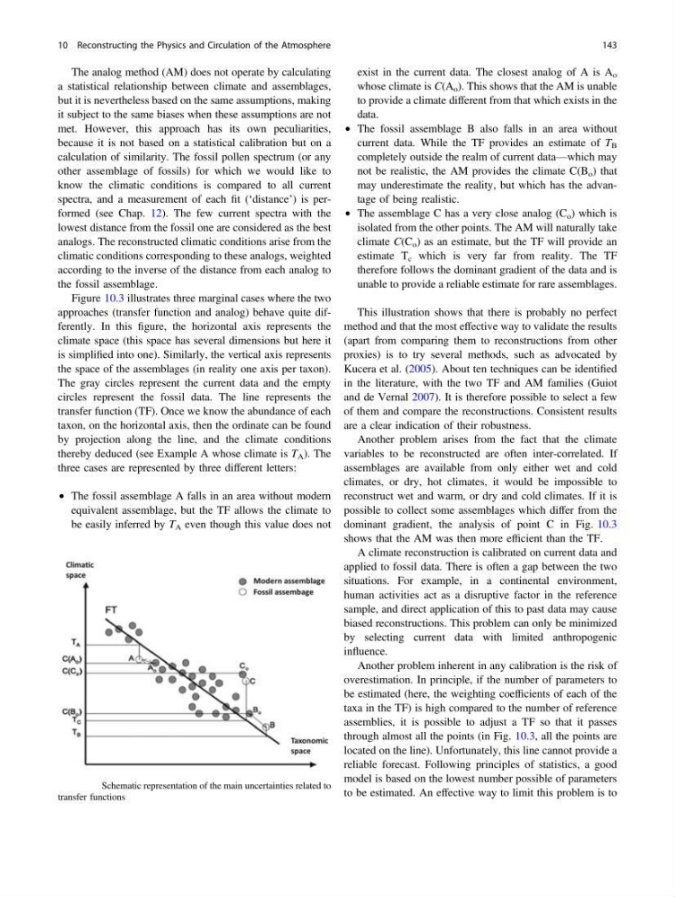
Figure 10.3 illustrates three marginal cases where the two
approaches (transfer function and analog) behave quite differently. In this figure, the horizontal axis represents the
climate space (this space has several dimensions but here it
is simplified into one). Similarly, the vertical axis represents
the space of the assemblages (in reality one axis per taxon).
The gray circles represent the current data and the empty
circles represent the fossil data. The line represents the
transfer function (TF). Once we know the abundance of each
taxon, on the horizontal axis, then the ordinate can be found
by projection along the line, and the climate conditions
thereby deduced (see Example A whose climate is T A ). The
three cases are represented by three different letters:
• The fossil assemblage A falls in an area without modern
equivalent assemblage, but the TF allows the climate to
be easily inferred by T A even though this value does not
exist in the current data. The closest analog of A is A o
whose climate is C(A o ). This shows that the AM is unable
to provide a climate different from that which exists in the
data.
• The fossil assemblage B also falls in an area without
current data. While the TF provides an estimate of T B
completely outside the realm of current data—which may
not be realistic, the AM provides the climate C(B o ) that
may underestimate the reality, but which has the advantage of being realistic.
• The assemblage C has a very close analog (C o ) which is
isolated from the other points. The AM will naturally take
climate C(C o ) as an estimate, but the TF will provide an
estimate T c which is very far from reality. The TF
therefore follows the dominant gradient of the data and is
unable to provide a reliable estimate for rare assemblages.
This illustration shows that there is probably no perfect
method and that the most effective way to validate the results
(apart from comparing them to reconstructions from other
proxies) is to try several methods, such as advocated by
Kucera et al. (2005). About ten techniques can be identified
in the literature, with the two TF and AM families (Guiot
and de Vernal 2007). It is therefore possible to select a few
of them and compare the reconstructions. Consistent results
are a clear indication of their robustness.
Another problem arises from the fact that the climate
variables to be reconstructed are often inter-correlated. If
assemblages are available from only either wet and cold
climates, or dry, hot climates, it would be impossible to
reconstruct wet and warm, or dry and cold climates. If it is
possible to collect some assemblages which differ from the
dominant gradient, the analysis of point C in Fig. 10.3
shows that the AM was then more efficient than the TF.
A climate reconstruction is calibrated on current data and
applied to fossil data. There is often a gap between the two
situations. For example, in a continental environment,
human activities act as a disruptive factor in the reference
sample, and direct application of this to past data may cause
biased reconstructions. This problem can only be minimized
by selecting current data with limited anthropogenic
influence.
Another problem inherent in any calibration is the risk of
overestimation. In principle, if the number of parameters to
be estimated (here, the weighting coefficients of each of the
taxa in the TF) is high compared to the number of reference
assemblies, it is possible to adjust a TF so that it passes
through almost all the points (in Fig. 10.3, all the points are
located on the line). Unfortunately, this line cannot provide a
reliable forecast. Following principles of statistics, a good
model is based on the lowest number possible of parameters
to be estimated. An effective way to limit this problem is to
Fig. 10.3 Schematic representation of the main uncertainties related to
transfer functions
10 Reconstructing the Physics and Circulation of the Atmosphere
143
a statistical relationship between climate and assemblages,
but it is nevertheless based on the same assumptions, making
it subject to the same biases when these assumptions are not
met. However, this approach has its own peculiarities,
because it is not based on a statistical calibration but on a
calculation of similarity. The fossil pollen spectrum (or any
other assemblage of fossils) for which we would like to
know the climatic conditions is compared to all current
spectra, and a measurement of each fit (‘distance’) is performed (see Chap. 12). The few current spectra with the
lowest distance from the fossil one are considered as the best
analogs. The reconstructed climatic conditions arise from the
climatic conditions corresponding to these analogs, weighted
according to the inverse of the distance from each analog to
the fossil assemblage.
Figure 10.3 illustrates three marginal cases where the two
approaches (transfer function and analog) behave quite differently. In this figure, the horizontal axis represents the
climate space (this space has several dimensions but here it
is simplified into one). Similarly, the vertical axis represents
the space of the assemblages (in reality one axis per taxon).
The gray circles represent the current data and the empty
circles represent the fossil data. The line represents the
transfer function (TF). Once we know the abundance of each
taxon, on the horizontal axis, then the ordinate can be found
by projection along the line, and the climate conditions
thereby deduced (see Example A whose climate is T A ). The
three cases are represented by three different letters:
• The fossil assemblage A falls in an area without modern
equivalent assemblage, but the TF allows the climate to
be easily inferred by T A even though this value does not
exist in the current data. The closest analog of A is A o
whose climate is C(A o ). This shows that the AM is unable
to provide a climate different from that which exists in the
data.
• The fossil assemblage B also falls in an area without
current data. While the TF provides an estimate of T B
completely outside the realm of current data—which may
not be realistic, the AM provides the climate C(B o ) that
may underestimate the reality, but which has the advantage of being realistic.
• The assemblage C has a very close analog (C o ) which is
isolated from the other points. The AM will naturally take
climate C(C o ) as an estimate, but the TF will provide an
estimate T c which is very far from reality. The TF
therefore follows the dominant gradient of the data and is
unable to provide a reliable estimate for rare assemblages.
This illustration shows that there is probably no perfect
method and that the most effective way to validate the results
(apart from comparing them to reconstructions from other
proxies) is to try several methods, such as advocated by
Kucera et al. (2005). About ten techniques can be identified
in the literature, with the two TF and AM families (Guiot
and de Vernal 2007). It is therefore possible to select a few
of them and compare the reconstructions. Consistent results
are a clear indication of their robustness.
Another problem arises from the fact that the climate
variables to be reconstructed are often inter-correlated. If
assemblages are available from only either wet and cold
climates, or dry, hot climates, it would be impossible to
reconstruct wet and warm, or dry and cold climates. If it is
possible to collect some assemblages which differ from the
dominant gradient, the analysis of point C in Fig. 10.3
shows that the AM was then more efficient than the TF.
A climate reconstruction is calibrated on current data and
applied to fossil data. There is often a gap between the two
situations. For example, in a continental environment,
human activities act as a disruptive factor in the reference
sample, and direct application of this to past data may cause
biased reconstructions. This problem can only be minimized
by selecting current data with limited anthropogenic
influence.
Another problem inherent in any calibration is the risk of
overestimation. In principle, if the number of parameters to
be estimated (here, the weighting coefficients of each of the
taxa in the TF) is high compared to the number of reference
assemblies, it is possible to adjust a TF so that it passes
through almost all the points (in Fig. 10.3, all the points are
located on the line). Unfortunately, this line cannot provide a
reliable forecast. Following principles of statistics, a good
model is based on the lowest number possible of parameters
to be estimated. An effective way to limit this problem is to
Fig. 10.3 Schematic representation of the main uncertainties related to
transfer functions
10 Reconstructing the Physics and Circulation of the Atmosphere
143