

272
M. Sato
ˆ
H
(2)
= ˆ
P −n
∞
m=1
j
ˆ
H +m | −(n+m) j j −(n+m) | ˆ
H −m
nω − (n + m)ω
+
j
ˆ
H −m | −(n−m) j j −(n−m) | ˆ
H +m
nω − (n − m)ω
ˆ
P −n .
(11.14)
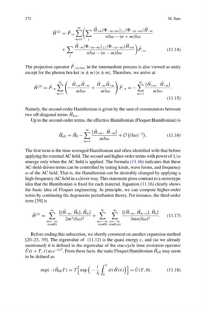
The projection operator ˆ
P −(n±m) in the intermediate process is also viewed as unity
except for the photon bra-ket |n ± mn ± m|. Therefore, we arrive at
ˆ
H
(2)
= ˆ
P −n
∞
m=1
−
ˆ
H +m ˆ
H −m
mω
+
ˆ
H −m ˆ
H +m
mω
ˆ
P −n = −
∞
m=1
[ ˆ
H +m , ˆ
H −m ]
mω
.
(11.15)
Namely, the second-order Hamiltonian is given by the sum of commutators between
two off-diagonal terms ˆ
H ±m .
Up to the second-order terms, the effective Hamiltonian (Floquet Hamiltonian) is
ˆ
H eff = ˆ
H 0 −
∞
m=1
[ ˆ
H +m , ˆ
H −m ]
mω
+ O
(ω)
−2
.
(11.16)
The first term is the time averaged Hamiltonian and often identified with that before
applying the external AC field. The second and higher-order terms with power of 1/ω
emerge only when the AC field is applied. The formula (11.16) indicates that these
AC-field-driven terms can be controlled by tuning kinds, wave forms, and frequency
ω of the AC field. That is, the Hamiltonian can be desirably changed by applying a
high-frequency AC field in a clever way. This statement gives contrast to a stereotype
idea that the Hamiltonian is fixed for each material. Equation (11.16) clearly shows
the basic idea of Floquet engineering. In principle, we can compute higher-order
terms by continuing the degenerate perturbation theory. For instance, the third-order
term [39] is
ˆ
H
(3)
=
∞
m=−∞
(m =0)
[[ ˆ
H −m , ˆ
H 0 ], ˆ
H m ]
2m 2 (ω) 2
+
∞
m=−∞
(m =0)
∞
n=−∞
(n =0,m)
[[ ˆ
H −m , ˆ
H m−n ], ˆ
H n ]
3mn(ω) 2
. (11.17)
Before ending this subsection, we shortly comment on another expansion method
[20–23, 39]. The eigenvalue of (11.12) is the quasi energy , and (as we already
mentioned) it is defined in the eigenvalue of the one-cycle time evolution operator
ˆ
U (t + T, t) as e
−iT . From these facts, the static Floquet Hamiltonian ˆ
H eff may seem
to be defined as
exp(−i ˆ
H eff T ) = T
exp
−
i
T
0
dτ ˆ
H (τ )
= ˆ
U (T, 0).
(11.18)
M. Sato
ˆ
H
(2)
= ˆ
P −n
∞
m=1
j
ˆ
H +m | −(n+m) j j −(n+m) | ˆ
H −m
nω − (n + m)ω
+
j
ˆ
H −m | −(n−m) j j −(n−m) | ˆ
H +m
nω − (n − m)ω
ˆ
P −n .
(11.14)
The projection operator ˆ
P −(n±m) in the intermediate process is also viewed as unity
except for the photon bra-ket |n ± mn ± m|. Therefore, we arrive at
ˆ
H
(2)
= ˆ
P −n
∞
m=1
−
ˆ
H +m ˆ
H −m
mω
+
ˆ
H −m ˆ
H +m
mω
ˆ
P −n = −
∞
m=1
[ ˆ
H +m , ˆ
H −m ]
mω
.
(11.15)
Namely, the second-order Hamiltonian is given by the sum of commutators between
two off-diagonal terms ˆ
H ±m .
Up to the second-order terms, the effective Hamiltonian (Floquet Hamiltonian) is
ˆ
H eff = ˆ
H 0 −
∞
m=1
[ ˆ
H +m , ˆ
H −m ]
mω
+ O
(ω)
−2
.
(11.16)
The first term is the time averaged Hamiltonian and often identified with that before
applying the external AC field. The second and higher-order terms with power of 1/ω
emerge only when the AC field is applied. The formula (11.16) indicates that these
AC-field-driven terms can be controlled by tuning kinds, wave forms, and frequency
ω of the AC field. That is, the Hamiltonian can be desirably changed by applying a
high-frequency AC field in a clever way. This statement gives contrast to a stereotype
idea that the Hamiltonian is fixed for each material. Equation (11.16) clearly shows
the basic idea of Floquet engineering. In principle, we can compute higher-order
terms by continuing the degenerate perturbation theory. For instance, the third-order
term [39] is
ˆ
H
(3)
=
∞
m=−∞
(m =0)
[[ ˆ
H −m , ˆ
H 0 ], ˆ
H m ]
2m 2 (ω) 2
+
∞
m=−∞
(m =0)
∞
n=−∞
(n =0,m)
[[ ˆ
H −m , ˆ
H m−n ], ˆ
H n ]
3mn(ω) 2
. (11.17)
Before ending this subsection, we shortly comment on another expansion method
[20–23, 39]. The eigenvalue of (11.12) is the quasi energy , and (as we already
mentioned) it is defined in the eigenvalue of the one-cycle time evolution operator
ˆ
U (t + T, t) as e
−iT . From these facts, the static Floquet Hamiltonian ˆ
H eff may seem
to be defined as
exp(−i ˆ
H eff T ) = T
exp
−
i
T
0
dτ ˆ
H (τ )
= ˆ
U (T, 0).
(11.18)