

9 Symmetry Approach to Chiral Optomagnonics in Antiferromagnetic Insulators
221
The resulting equation of motion for ˜
ψ is given by (9.45) with the diagonal matrix
on the right-hand side
˜
H 0 = U
†
m H 0 U m = diag(−ω p , ω p , 0, ω p , −ω p , 0).
(9.48)
This describes two antiferromagnetic spin waves with an energy dispersion ω p degenerate with respect to the two polarization states. In an antiferromagnet, magnetization
precession is locked in the real space to the direction of n, so that these polarization
states correspond to left and right circular polarizations along the anisotropy axis.
This is in contrast to electrodynamics, where we deal with real helicity—precession
around the direction of wave vector p.
Secondly, we have to find all the matrices Q that commute with ˜
H 0 , which can
be done precisely in the same way as in (9.17). It should be mentioned that in the
region (α − α
) p
2
β, antiferromagnetic spin waves have almost linear dispersion,
ω p = c s p, where the velocity is given by c s = γ M s
√ δ(α − α ). This fact gives them
the appearance similar to the electromagnetic waves. However, we emphasize that
the linear dispersion is not essential for our symmetry analysis.
What is important is that the eigenvalues of ˜
H 0 are degenerate. This fact allows
us find the eight-dimensional algebra of the symmetry transformations, which is
isomorphic to invariance algebra of the Maxwell’s equations. The generators of this
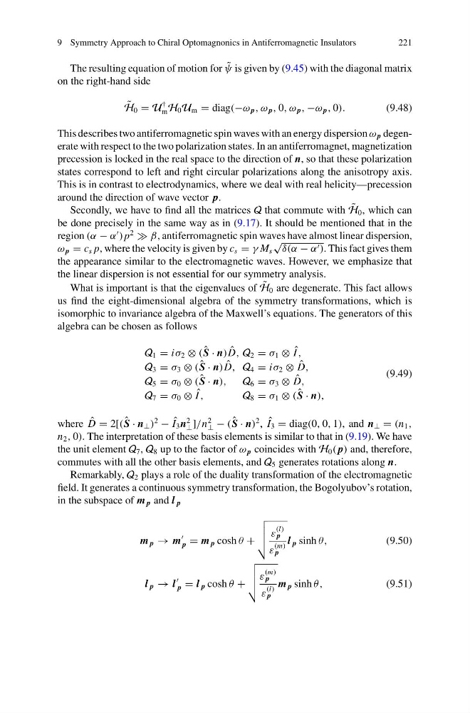
algebra can be chosen as follows
Q 1 = iσ 2 ⊗ ( ˆ
S · n) ˆ
D, Q 2 = σ 1 ⊗ ˆ
I ,
Q 3 = σ 3 ⊗ ( ˆ
S · n) ˆ
D, Q 4 = iσ 2 ⊗ ˆ
D,
Q 5 = σ 0 ⊗ ( ˆ
S · n),
Q 6 = σ 3 ⊗ ˆ
D,
Q 7 = σ 0 ⊗ ˆ
I ,
Q 8 = σ 1 ⊗ ( ˆ
S · n),
(9.49)
where ˆ
D = 2[( ˆ
S · n ⊥ )
2
− ˆ
I 3 n
2
⊥ ]/n
2
⊥ − ( ˆ
S · n)
2 , ˆ
I 3 = diag(0, 0, 1), and n ⊥ = (n 1 ,
n 2 , 0). The interpretation of these basis elements is similar to that in (9.19). We have
the unit element Q 7 , Q 8 up to the factor of ω p coincides with H 0 ( p) and, therefore,
commutes with all the other basis elements, and Q 5 generates rotations along n.
Remarkably, Q 2 plays a role of the duality transformation of the electromagnetic
field. It generates a continuous symmetry transformation, the Bogolyubov’s rotation,
in the subspace of m p and l p
m p → m
p = m p cosh θ +
ε
(l)
p
ε
(m)
p
l p sinh θ,
(9.50)
l p → l
p = l p cosh θ +
ε
(m)
p
ε
(l)
p
m p sinh θ,
(9.51)
221
The resulting equation of motion for ˜
ψ is given by (9.45) with the diagonal matrix
on the right-hand side
˜
H 0 = U
†
m H 0 U m = diag(−ω p , ω p , 0, ω p , −ω p , 0).
(9.48)
This describes two antiferromagnetic spin waves with an energy dispersion ω p degenerate with respect to the two polarization states. In an antiferromagnet, magnetization
precession is locked in the real space to the direction of n, so that these polarization
states correspond to left and right circular polarizations along the anisotropy axis.
This is in contrast to electrodynamics, where we deal with real helicity—precession
around the direction of wave vector p.
Secondly, we have to find all the matrices Q that commute with ˜
H 0 , which can
be done precisely in the same way as in (9.17). It should be mentioned that in the
region (α − α
) p
2
β, antiferromagnetic spin waves have almost linear dispersion,
ω p = c s p, where the velocity is given by c s = γ M s
√ δ(α − α ). This fact gives them
the appearance similar to the electromagnetic waves. However, we emphasize that
the linear dispersion is not essential for our symmetry analysis.
What is important is that the eigenvalues of ˜
H 0 are degenerate. This fact allows
us find the eight-dimensional algebra of the symmetry transformations, which is
isomorphic to invariance algebra of the Maxwell’s equations. The generators of this
algebra can be chosen as follows
Q 1 = iσ 2 ⊗ ( ˆ
S · n) ˆ
D, Q 2 = σ 1 ⊗ ˆ
I ,
Q 3 = σ 3 ⊗ ( ˆ
S · n) ˆ
D, Q 4 = iσ 2 ⊗ ˆ
D,
Q 5 = σ 0 ⊗ ( ˆ
S · n),
Q 6 = σ 3 ⊗ ˆ
D,
Q 7 = σ 0 ⊗ ˆ
I ,
Q 8 = σ 1 ⊗ ( ˆ
S · n),
(9.49)
where ˆ
D = 2[( ˆ
S · n ⊥ )
2
− ˆ
I 3 n
2
⊥ ]/n
2
⊥ − ( ˆ
S · n)
2 , ˆ
I 3 = diag(0, 0, 1), and n ⊥ = (n 1 ,
n 2 , 0). The interpretation of these basis elements is similar to that in (9.19). We have
the unit element Q 7 , Q 8 up to the factor of ω p coincides with H 0 ( p) and, therefore,
commutes with all the other basis elements, and Q 5 generates rotations along n.
Remarkably, Q 2 plays a role of the duality transformation of the electromagnetic
field. It generates a continuous symmetry transformation, the Bogolyubov’s rotation,
in the subspace of m p and l p
m p → m
p = m p cosh θ +
ε
(l)
p
ε
(m)
p
l p sinh θ,
(9.50)
l p → l
p = l p cosh θ +
ε
(m)
p
ε
(l)
p
m p sinh θ,
(9.51)