

18 A Plausible Description of Continuum …
363
is on the right (Neumann’s condition) and no displacements on the left (Dirichlet
conditions).
The equations to be solved are:
Y
2(1 + ν)
∇
2 u +
Y
2(1 − ν)
∂
∂ x
u +
∂
∂ y
v
= 0
Y
2(1 + ν)
∇
2 v +
Y
2(1 − ν)
∂
∂ x
u +
∂
∂ y
v
= 0
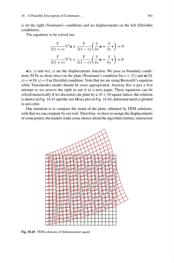
u(x, y) and v(x, y) are the displacements function. We pose as boundary conditions 50 Pa as shear stress on the plate (Neumann’s condition for x = 21) and u(10,
y) = v(10, y) = 0 as Dirichlet condition. Note that we are using Bernoulli’s equation
while Timoshenko model should be more appropriated. Anyway this is just a first
attempt so we reserve the right to use it in a next paper. These equations can be
solved numerically if we discretize our plate by a 10 × 10 square lattice; the solution
is shown in Fig. 18.43 and the von Mises plot in Fig. 18.44; deformed mesh is plotted
in red color.
Our intention is to compare the strain of the plate, obtained by FEM solutions,
with that we can compute by our tool. Therefore, we have to assign the displacements
of some points, the leaders make some choice about the algorithm (lattice, interaction
Fig. 18.43 FEM solutions of bidimensional square
363
is on the right (Neumann’s condition) and no displacements on the left (Dirichlet
conditions).
The equations to be solved are:
Y
2(1 + ν)
∇
2 u +
Y
2(1 − ν)
∂
∂ x
u +
∂
∂ y
v
= 0
Y
2(1 + ν)
∇
2 v +
Y
2(1 − ν)
∂
∂ x
u +
∂
∂ y
v
= 0
u(x, y) and v(x, y) are the displacements function. We pose as boundary conditions 50 Pa as shear stress on the plate (Neumann’s condition for x = 21) and u(10,
y) = v(10, y) = 0 as Dirichlet condition. Note that we are using Bernoulli’s equation
while Timoshenko model should be more appropriated. Anyway this is just a first
attempt so we reserve the right to use it in a next paper. These equations can be
solved numerically if we discretize our plate by a 10 × 10 square lattice; the solution
is shown in Fig. 18.43 and the von Mises plot in Fig. 18.44; deformed mesh is plotted
in red color.
Our intention is to compare the strain of the plate, obtained by FEM solutions,
with that we can compute by our tool. Therefore, we have to assign the displacements
of some points, the leaders make some choice about the algorithm (lattice, interaction
Fig. 18.43 FEM solutions of bidimensional square