

17 Microplane Modeling for Inelastic Responses …
317
experimental case, performed by Reedlunn et al. (2014), is reported here and readers
are referred to (Karamooz Ravari et al. 2015) for more information and case studies.
The experimental measurements, presented in Reedlunn et al. (2014), were
performed isothermally using cold-drawn, slightly Ni-rich NiTi tube from Memry
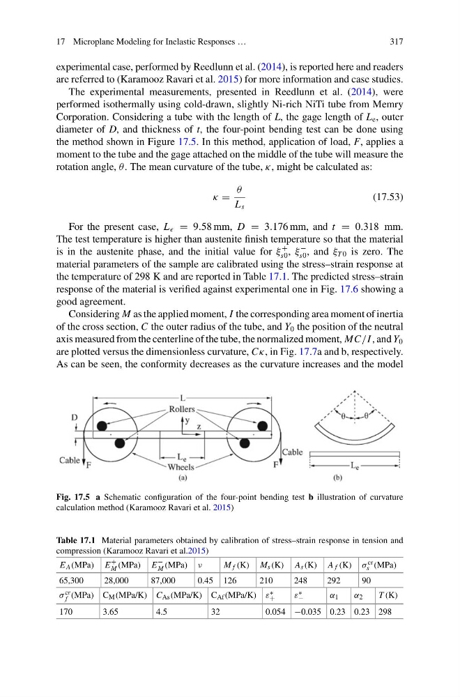
Corporation. Considering a tube with the length of L, the gage length of L e , outer
diameter of D, and thickness of t, the four-point bending test can be done using
the method shown in Figure 17.5. In this method, application of load, F, applies a
moment to the tube and the gage attached on the middle of the tube will measure the
rotation angle, θ . The mean curvature of the tube, κ, might be calculated as:
κ =
θ
L s
(17.53)
For the present case, L e = 9.58 mm, D = 3.176 mm, and t = 0.318 mm.
The test temperature is higher than austenite finish temperature so that the material
is in the austenite phase, and the initial value for ξ
+
s0 , ξ
−
s0 , and ξ T 0 is zero. The
material parameters of the sample are calibrated using the stress–strain response at
the temperature of 298 K and are reported in Table 17.1. The predicted stress–strain
response of the material is verified against experimental one in Fig. 17.6 showing a
good agreement.
Considering M as the applied moment, I the corresponding area moment of inertia
of the cross section, C the outer radius of the tube, and Y 0 the position of the neutral
axis measured from the centerline of the tube, the normalized moment, MC/I , and Y 0
are plotted versus the dimensionless curvature, Cκ, in Fig. 17.7a and b, respectively.
As can be seen, the conformity decreases as the curvature increases and the model
Fig. 17.5 a Schematic configuration of the four-point bending test b illustration of curvature
calculation method (Karamooz Ravari et al. 2015)
Table 17.1 Material parameters obtained by calibration of stress–strain response in tension and
compression (Karamooz Ravari et al.2015)
E A (MPa) E
+
M (MPa) E
−
M (MPa) ν
M f (K) M s (K) A s (K) A f (K) σ cr
s (MPa)
65,300
28,000
87,000
0.45 126
210
248
292
90
σ cr
f (MPa) C M (MPa/K) C As (MPa/K) C Af (MPa/K) ε ∗
+
ε ∗
−
α 1
α 2
T (K)
170
3.65
4.5
32
0.054 −0.035 0.23 0.23 298
317
experimental case, performed by Reedlunn et al. (2014), is reported here and readers
are referred to (Karamooz Ravari et al. 2015) for more information and case studies.
The experimental measurements, presented in Reedlunn et al. (2014), were
performed isothermally using cold-drawn, slightly Ni-rich NiTi tube from Memry
Corporation. Considering a tube with the length of L, the gage length of L e , outer
diameter of D, and thickness of t, the four-point bending test can be done using
the method shown in Figure 17.5. In this method, application of load, F, applies a
moment to the tube and the gage attached on the middle of the tube will measure the
rotation angle, θ . The mean curvature of the tube, κ, might be calculated as:
κ =
θ
L s
(17.53)
For the present case, L e = 9.58 mm, D = 3.176 mm, and t = 0.318 mm.
The test temperature is higher than austenite finish temperature so that the material
is in the austenite phase, and the initial value for ξ
+
s0 , ξ
−
s0 , and ξ T 0 is zero. The
material parameters of the sample are calibrated using the stress–strain response at
the temperature of 298 K and are reported in Table 17.1. The predicted stress–strain
response of the material is verified against experimental one in Fig. 17.6 showing a
good agreement.
Considering M as the applied moment, I the corresponding area moment of inertia
of the cross section, C the outer radius of the tube, and Y 0 the position of the neutral
axis measured from the centerline of the tube, the normalized moment, MC/I , and Y 0
are plotted versus the dimensionless curvature, Cκ, in Fig. 17.7a and b, respectively.
As can be seen, the conformity decreases as the curvature increases and the model
Fig. 17.5 a Schematic configuration of the four-point bending test b illustration of curvature
calculation method (Karamooz Ravari et al. 2015)
Table 17.1 Material parameters obtained by calibration of stress–strain response in tension and
compression (Karamooz Ravari et al.2015)
E A (MPa) E
+
M (MPa) E
−
M (MPa) ν
M f (K) M s (K) A s (K) A f (K) σ cr
s (MPa)
65,300
28,000
87,000
0.45 126
210
248
292
90
σ cr
f (MPa) C M (MPa/K) C As (MPa/K) C Af (MPa/K) ε ∗
+
ε ∗
−
α 1
α 2
T (K)
170
3.65
4.5
32
0.054 −0.035 0.23 0.23 298