

114
L. Igumnov et al.
8.3 Motion Equation of Soil
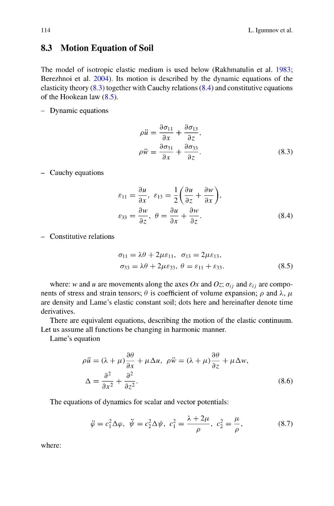
The model of isotropic elastic medium is used below (Rakhmatulin et al. 1983;
Berezhnoi et al. 2004). Its motion is described by the dynamic equations of the
elasticity theory (8.3) together with Cauchy relations (8.4) and constitutive equations
of the Hookean law (8.5).
– Dynamic equations
ρ ¨
u =
∂σ 11
∂ x
+
∂σ 13
∂z
,
ρ ¨
w =
∂σ 31
∂ x
+
∂σ 33
∂z
.
(8.3)
– Cauchy equations
ε 11 =
∂u
∂ x
, ε 13 =
1
2
∂u
∂z
+
∂w
∂ x
,
ε 33 =
∂w
∂z
, θ =
∂u
∂ x
+
∂w
∂z
.
(8.4)
– Constitutive relations
σ 11 = λθ + 2με 11 , σ 13 = 2με 13 ,
σ 33 = λθ + 2με 33 , θ = ε 11 + ε 33 .
(8.5)
where: w and u are movements along the axes Ox and Oz; σ i j and ε i j are components of stress and strain tensors; θ is coefficient of volume expansion; ρ and λ, μ
are density and Lame’s elastic constant soil; dots here and hereinafter denote time
derivatives.
There are equivalent equations, describing the motion of the elastic continuum.
Let us assume all functions be changing in harmonic manner.
Lame’s equation
ρ ¨
u = (λ + μ)
∂θ
∂ x
+ μμu, ρ ¨
w = (λ + μ)
∂θ
∂z
+ μμw,
=
∂
2
∂ x 2 +
∂
2
∂z 2 .
(8.6)
The equations of dynamics for scalar and vector potentials:
¨
ϕ = c
2
1 ¨
ψ = c
2
2 c
2
1 =
λ + 2μ
ρ
, c
2
2 =
μ
ρ
,
(8.7)
where:
L. Igumnov et al.
8.3 Motion Equation of Soil
The model of isotropic elastic medium is used below (Rakhmatulin et al. 1983;
Berezhnoi et al. 2004). Its motion is described by the dynamic equations of the
elasticity theory (8.3) together with Cauchy relations (8.4) and constitutive equations
of the Hookean law (8.5).
– Dynamic equations
ρ ¨
u =
∂σ 11
∂ x
+
∂σ 13
∂z
,
ρ ¨
w =
∂σ 31
∂ x
+
∂σ 33
∂z
.
(8.3)
– Cauchy equations
ε 11 =
∂u
∂ x
, ε 13 =
1
2
∂u
∂z
+
∂w
∂ x
,
ε 33 =
∂w
∂z
, θ =
∂u
∂ x
+
∂w
∂z
.
(8.4)
– Constitutive relations
σ 11 = λθ + 2με 11 , σ 13 = 2με 13 ,
σ 33 = λθ + 2με 33 , θ = ε 11 + ε 33 .
(8.5)
where: w and u are movements along the axes Ox and Oz; σ i j and ε i j are components of stress and strain tensors; θ is coefficient of volume expansion; ρ and λ, μ
are density and Lame’s elastic constant soil; dots here and hereinafter denote time
derivatives.
There are equivalent equations, describing the motion of the elastic continuum.
Let us assume all functions be changing in harmonic manner.
Lame’s equation
ρ ¨
u = (λ + μ)
∂θ
∂ x
+ μμu, ρ ¨
w = (λ + μ)
∂θ
∂z
+ μμw,
=
∂
2
∂ x 2 +
∂
2
∂z 2 .
(8.6)
The equations of dynamics for scalar and vector potentials:
¨
ϕ = c
2
1 ¨
ψ = c
2
2 c
2
1 =
λ + 2μ
ρ
, c
2
2 =
μ
ρ
,
(8.7)
where: