

7 Features of Subsonic Stage of Contact Interaction …
101
σ
e
13
x 3 =0
= 0, σ
e
33
x 3 =0
= δ(x 1 )δ(α).
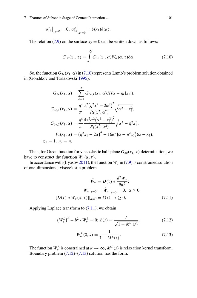
The relation (7.9) on the surface x 3 = 0 can be written down as follows:
G 30 (x 1 , τ ) =
∞
0
G 3e (x 1 , α)W σ (α, τ )dα.
(7.10)
So, the function G 3e (x 1 , α) in (7.10) represents Lamb’s problem solution obtained
in (Gorshkov and Tarlakovski 1995):
G 3e (x 1 , α) =
2
k=1
G 3e,k (x 1 , α)H (α − η k |x 1 |),
G 3e,1 (x 1 , α) =
η
4
π
x
2
1
η
2 x
2
1 − 2α
2
2
P 4 (x
2
1 , α 2 )
α 2 − x
2
1 ,
G 3e,2 (x 1 , α) =
η
4
π
4x
2
1 α
2
α
2
− x
2
1
2
P 4 (x
2
1 , α 2 )
α 2 − η 2 x
2
1 ,
P 4 (x 1 , α) =
η
2 x 1 − 2α
4 − 16α
2
α − η
2 x 1
(α − x 1 ),
η 1 = 1, η 2 = η.
Then, for Green function for viscoelastic half-plane G 30 (x 1 , τ ) determination, we
have to construct the function W σ (α, τ ).
In accordance with (Ilyasov 2011), the function W σ in (7.9) is constrained solution
of one-dimensional viscoelastic problem
¨
W σ = D(τ ) ∗
∂
2 W σ
∂α 2 ;
W σ | τ =0 = ˙
W σ
τ =0 = 0, α ≥ 0;
[D(τ ) ∗ W σ (α, τ )]| α=0 = δ(τ ), τ ≥ 0.
(7.11)
Applying Laplace transform to (7.11), we obtain
W
L
σ
− b
2
· W
L
σ = 0; b(s) =
s
1 − M L (s)
,
(7.12)
W
L
σ (0, s) =
1
1 − M L (s)
.
(7.13)
The function W
L
σ is constrained at α → ∞, M
L
(s) is relaxation kernel transform.
Boundary problem (7.12)–(7.13) solution has the form:
101
σ
e
13
x 3 =0
= 0, σ
e
33
x 3 =0
= δ(x 1 )δ(α).
The relation (7.9) on the surface x 3 = 0 can be written down as follows:
G 30 (x 1 , τ ) =
∞
0
G 3e (x 1 , α)W σ (α, τ )dα.
(7.10)
So, the function G 3e (x 1 , α) in (7.10) represents Lamb’s problem solution obtained
in (Gorshkov and Tarlakovski 1995):
G 3e (x 1 , α) =
2
k=1
G 3e,k (x 1 , α)H (α − η k |x 1 |),
G 3e,1 (x 1 , α) =
η
4
π
x
2
1
η
2 x
2
1 − 2α
2
2
P 4 (x
2
1 , α 2 )
α 2 − x
2
1 ,
G 3e,2 (x 1 , α) =
η
4
π
4x
2
1 α
2
α
2
− x
2
1
2
P 4 (x
2
1 , α 2 )
α 2 − η 2 x
2
1 ,
P 4 (x 1 , α) =
η
2 x 1 − 2α
4 − 16α
2
α − η
2 x 1
(α − x 1 ),
η 1 = 1, η 2 = η.
Then, for Green function for viscoelastic half-plane G 30 (x 1 , τ ) determination, we
have to construct the function W σ (α, τ ).
In accordance with (Ilyasov 2011), the function W σ in (7.9) is constrained solution
of one-dimensional viscoelastic problem
¨
W σ = D(τ ) ∗
∂
2 W σ
∂α 2 ;
W σ | τ =0 = ˙
W σ
τ =0 = 0, α ≥ 0;
[D(τ ) ∗ W σ (α, τ )]| α=0 = δ(τ ), τ ≥ 0.
(7.11)
Applying Laplace transform to (7.11), we obtain
W
L
σ
− b
2
· W
L
σ = 0; b(s) =
s
1 − M L (s)
,
(7.12)
W
L
σ (0, s) =
1
1 − M L (s)
.
(7.13)
The function W
L
σ is constrained at α → ∞, M
L
(s) is relaxation kernel transform.
Boundary problem (7.12)–(7.13) solution has the form: