

148
14 Difficulties of Radiological and Nuclear Interdiction
14.1.1 The Random Nature of Radioactive Decay
There are radiation instruments that will record every count received over a period
of time; if the user sets it to count for one minute then, at the end of one minute,
the display will show the total number of counts recorded from the time the “start”
button was pushed until one minute has elapsed. So consider a technician whose
job it is to push the button, record the number of counts, and then push the button
again. Over time the technician will note that, while readings will vary from one
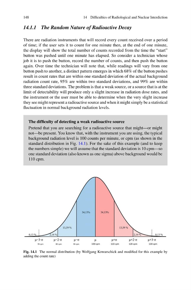
button push to another, a distinct pattern emerges in which 68% of the button pushes
result in count rates that are within one standard deviation of the actual background
radiation count rate, 95% are within two standard deviations, and 99% are within
three standard deviations. The problem is that a weak source, or a source that is at the
limit of detectability will produce only a slight increase in radiation dose rates, and
the instrument or the user must be able to determine when the very slight increase
they see might represent a radioactive source and when it might simply be a statistical
fluctuation in normal background radiation levels.
The difficulty of detecting a weak radioactive source
Pretend that you are searching for a radioactive source that might—or might
not—be present. You know that, with the instrument you are using, the typical
background radiation level is 100 counts per minute, or cpm (as shown in the
standard distribution in Fig. 14.1). For the sake of this example (and to keep
the numbers simple) we will assume that the standard deviation is 10 cpm—so
one standard deviation (also known as one sigma) above background would be
110 cpm.
Fig. 14.1 The normal distribution (by Wolfgang Kowarschick and modified for this example by
adding the count rate)
14 Difficulties of Radiological and Nuclear Interdiction
14.1.1 The Random Nature of Radioactive Decay
There are radiation instruments that will record every count received over a period
of time; if the user sets it to count for one minute then, at the end of one minute,
the display will show the total number of counts recorded from the time the “start”
button was pushed until one minute has elapsed. So consider a technician whose
job it is to push the button, record the number of counts, and then push the button
again. Over time the technician will note that, while readings will vary from one
button push to another, a distinct pattern emerges in which 68% of the button pushes
result in count rates that are within one standard deviation of the actual background
radiation count rate, 95% are within two standard deviations, and 99% are within
three standard deviations. The problem is that a weak source, or a source that is at the
limit of detectability will produce only a slight increase in radiation dose rates, and
the instrument or the user must be able to determine when the very slight increase
they see might represent a radioactive source and when it might simply be a statistical
fluctuation in normal background radiation levels.
The difficulty of detecting a weak radioactive source
Pretend that you are searching for a radioactive source that might—or might
not—be present. You know that, with the instrument you are using, the typical
background radiation level is 100 counts per minute, or cpm (as shown in the
standard distribution in Fig. 14.1). For the sake of this example (and to keep
the numbers simple) we will assume that the standard deviation is 10 cpm—so
one standard deviation (also known as one sigma) above background would be
110 cpm.
Fig. 14.1 The normal distribution (by Wolfgang Kowarschick and modified for this example by
adding the count rate)