

7.8 State Reduction in the CHSH Scenario
139
λ
i j =
1
2
λ 0 j + λ 1 j + (−1)
i
(λ 0 j − λ 1 j ) cos[θ j (θ A , θ B )] + 2(−1)
i s j sin[θ j (θ A , θ B )]
(7.86)
s
j =s j cos[θ j (θ A , θ B )] −
1
2
(λ 0 j − λ 1 j ) sin[θ j (θ A , θ B )],
(7.87)
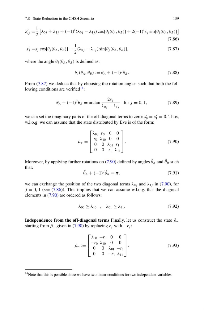
where the angle θ j (θ A , θ B ) is defined as:
θ j (θ A , θ B ) := θ A + (−1)
j
θ B .
(7.88)
From (7.87) we deduce that by choosing the rotation angles such that both the following conditions are verified
14 :
θ A + (−1)
j
θ B = arctan
2s j
λ 0 j − λ 1 j
for j = 0, 1,
(7.89)
we can set the imaginary parts of the off-diagonal terms to zero: s
0 = s
1 = 0. Thus,
w.l.o.g. we can assume that the state distributed by Eve is of the form:
¯
ρ + =
⎡
⎢
⎢
⎣
λ 00 r 0 0 0
r 0 λ 10 0 0
0 0 λ 01 r 1
0 0 r 1 λ 11
⎤
⎥
⎥
⎦ .
(7.90)
Moreover, by applying further rotations on (7.90) defined by angles ˜
θ A and ˜
θ B such
that:
˜
θ A + (−1)
j ˜
θ B = π,
(7.91)
we can exchange the position of the two diagonal terms λ 0 j and λ 1 j in (7.90), for
j = 0, 1 (see (7.86)). This implies that we can assume w.l.o.g. that the diagonal
elements in (7.90) are ordered as follows:
λ 00 ≥ λ 10 , λ 01 ≥ λ 11 .
(7.92)
Independence from the off-diagonal terms Finally, let us construct the state ¯
ρ −
starting from ¯
ρ + given in (7.90) by replacing r j with −r j :
¯
ρ − :=
⎡
⎢
⎢
⎣
λ 00 −r 0 0 0
−r 0 λ 10 0 0
0 0 λ 01 −r 1
0 0 −r 1 λ 11
⎤
⎥
⎥
⎦ .
(7.93)
14 Note that this is possible since we have two linear conditions for two independent variables.
139
λ
i j =
1
2
λ 0 j + λ 1 j + (−1)
i
(λ 0 j − λ 1 j ) cos[θ j (θ A , θ B )] + 2(−1)
i s j sin[θ j (θ A , θ B )]
(7.86)
s
j =s j cos[θ j (θ A , θ B )] −
1
2
(λ 0 j − λ 1 j ) sin[θ j (θ A , θ B )],
(7.87)
where the angle θ j (θ A , θ B ) is defined as:
θ j (θ A , θ B ) := θ A + (−1)
j
θ B .
(7.88)
From (7.87) we deduce that by choosing the rotation angles such that both the following conditions are verified
14 :
θ A + (−1)
j
θ B = arctan
2s j
λ 0 j − λ 1 j
for j = 0, 1,
(7.89)
we can set the imaginary parts of the off-diagonal terms to zero: s
0 = s
1 = 0. Thus,
w.l.o.g. we can assume that the state distributed by Eve is of the form:
¯
ρ + =
⎡
⎢
⎢
⎣
λ 00 r 0 0 0
r 0 λ 10 0 0
0 0 λ 01 r 1
0 0 r 1 λ 11
⎤
⎥
⎥
⎦ .
(7.90)
Moreover, by applying further rotations on (7.90) defined by angles ˜
θ A and ˜
θ B such
that:
˜
θ A + (−1)
j ˜
θ B = π,
(7.91)
we can exchange the position of the two diagonal terms λ 0 j and λ 1 j in (7.90), for
j = 0, 1 (see (7.86)). This implies that we can assume w.l.o.g. that the diagonal
elements in (7.90) are ordered as follows:
λ 00 ≥ λ 10 , λ 01 ≥ λ 11 .
(7.92)
Independence from the off-diagonal terms Finally, let us construct the state ¯
ρ −
starting from ¯
ρ + given in (7.90) by replacing r j with −r j :
¯
ρ − :=
⎡
⎢
⎢
⎣
λ 00 −r 0 0 0
−r 0 λ 10 0 0
0 0 λ 01 −r 1
0 0 −r 1 λ 11
⎤
⎥
⎥
⎦ .
(7.93)
14 Note that this is possible since we have two linear conditions for two independent variables.