

3 Uncertainty Quantification in Lasso-Type Regularization Problems
83
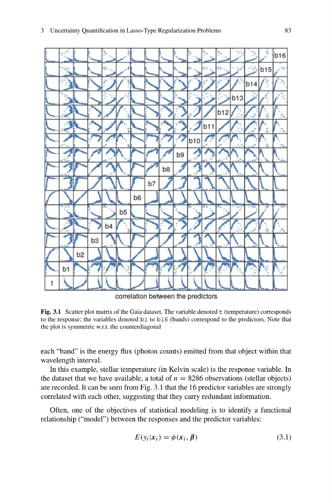
Fig. 3.1 Scatter plot matrix of the Gaia dataset. The variable denoted t (temperature) corresponds
to the response; the variables denoted b1 to b16 (bands) correspond to the predictors. Note that
the plot is symmetric w.r.t. the counterdiagonal
each “band” is the energy flux (photon counts) emitted from that object within that
wavelength interval.
In this example, stellar temperature (in Kelvin scale) is the response variable. In
the dataset that we have available, a total of n = 8286 observations (stellar objects)
are recorded. It can be seen from Fig. 3.1 that the 16 predictor variables are strongly
correlated with each other, suggesting that they carry redundant information.
Often, one of the objectives of statistical modeling is to identify a functional
relationship (“model”) between the responses and the predictor variables:
E(y i |x i ) = φ(x i , β)
(3.1)
83
Fig. 3.1 Scatter plot matrix of the Gaia dataset. The variable denoted t (temperature) corresponds
to the response; the variables denoted b1 to b16 (bands) correspond to the predictors. Note that
the plot is symmetric w.r.t. the counterdiagonal
each “band” is the energy flux (photon counts) emitted from that object within that
wavelength interval.
In this example, stellar temperature (in Kelvin scale) is the response variable. In
the dataset that we have available, a total of n = 8286 observations (stellar objects)
are recorded. It can be seen from Fig. 3.1 that the 16 predictor variables are strongly
correlated with each other, suggesting that they carry redundant information.
Often, one of the objectives of statistical modeling is to identify a functional
relationship (“model”) between the responses and the predictor variables:
E(y i |x i ) = φ(x i , β)
(3.1)