

2 Introduction to Imprecise Probabilities
73
Example 2.7 (continued)
the set of all exponential distributions. But now, we will employ a Bayesian
procedure where we model our knowledge about distribution parameter θ by
a probability distribution instead of selecting just one best-fit value.
First, a prior distribution π 0 (dλ), which represents our knowledge about λ
before observing the data, has to be elicited. Then, our knowledge is refined
via the Bayes updating rule to construct our posterior knowledge about θ as
w(θ) = p(θ|| x) ∝ L(θ ; ;
x)p 0 (θ ).
(2.27)
Equation (2.27) specifies the posterior probability density function (the
mixing weight) up to a normalisation constant. From that, we can construct
the predictive distribution for a future sample X n+1 as a weighted average of
predictions of all the models in P. Thus,
p(x n+1 || x) =
θ p(x n+1 |θ)p(θ|| x)dθ
Z( x)
,
(2.28)
where Z( x) is a normalisation constant.
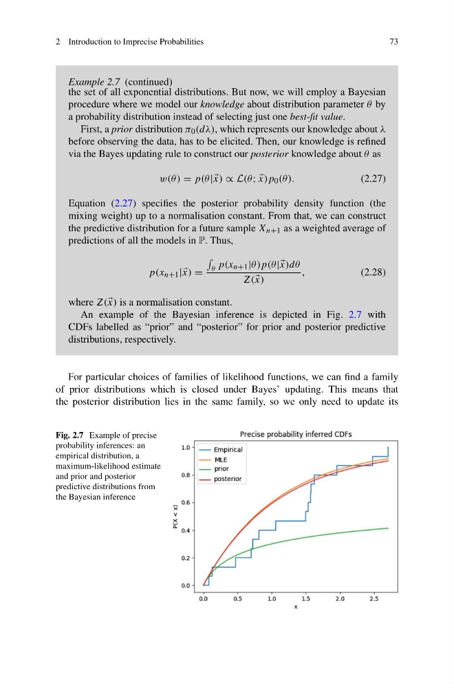
An example of the Bayesian inference is depicted in Fig. 2.7 with
CDFs labelled as “prior” and “posterior” for prior and posterior predictive
distributions, respectively.
For particular choices of families of likelihood functions, we can find a family
of prior distributions which is closed under Bayes’ updating. This means that
the posterior distribution lies in the same family, so we only need to update its
Fig. 2.7 Example of precise
probability inferences: an
empirical distribution, a
maximum-likelihood estimate
and prior and posterior
predictive distributions from
the Bayesian inference
73
Example 2.7 (continued)
the set of all exponential distributions. But now, we will employ a Bayesian
procedure where we model our knowledge about distribution parameter θ by
a probability distribution instead of selecting just one best-fit value.
First, a prior distribution π 0 (dλ), which represents our knowledge about λ
before observing the data, has to be elicited. Then, our knowledge is refined
via the Bayes updating rule to construct our posterior knowledge about θ as
w(θ) = p(θ|| x) ∝ L(θ ; ;
x)p 0 (θ ).
(2.27)
Equation (2.27) specifies the posterior probability density function (the
mixing weight) up to a normalisation constant. From that, we can construct
the predictive distribution for a future sample X n+1 as a weighted average of
predictions of all the models in P. Thus,
p(x n+1 || x) =
θ p(x n+1 |θ)p(θ|| x)dθ
Z( x)
,
(2.28)
where Z( x) is a normalisation constant.
An example of the Bayesian inference is depicted in Fig. 2.7 with
CDFs labelled as “prior” and “posterior” for prior and posterior predictive
distributions, respectively.
For particular choices of families of likelihood functions, we can find a family
of prior distributions which is closed under Bayes’ updating. This means that
the posterior distribution lies in the same family, so we only need to update its
Fig. 2.7 Example of precise
probability inferences: an
empirical distribution, a
maximum-likelihood estimate
and prior and posterior
predictive distributions from
the Bayesian inference