

68
D. Krpelík and T. Basu
max
a∈R
a
subject to,
a+
n
i=1
λ i [g i (x j ) − P (g i )] ≤ g(x j )
λ i ≥ 0 i = 1, 2, . . . , n
(2.19)
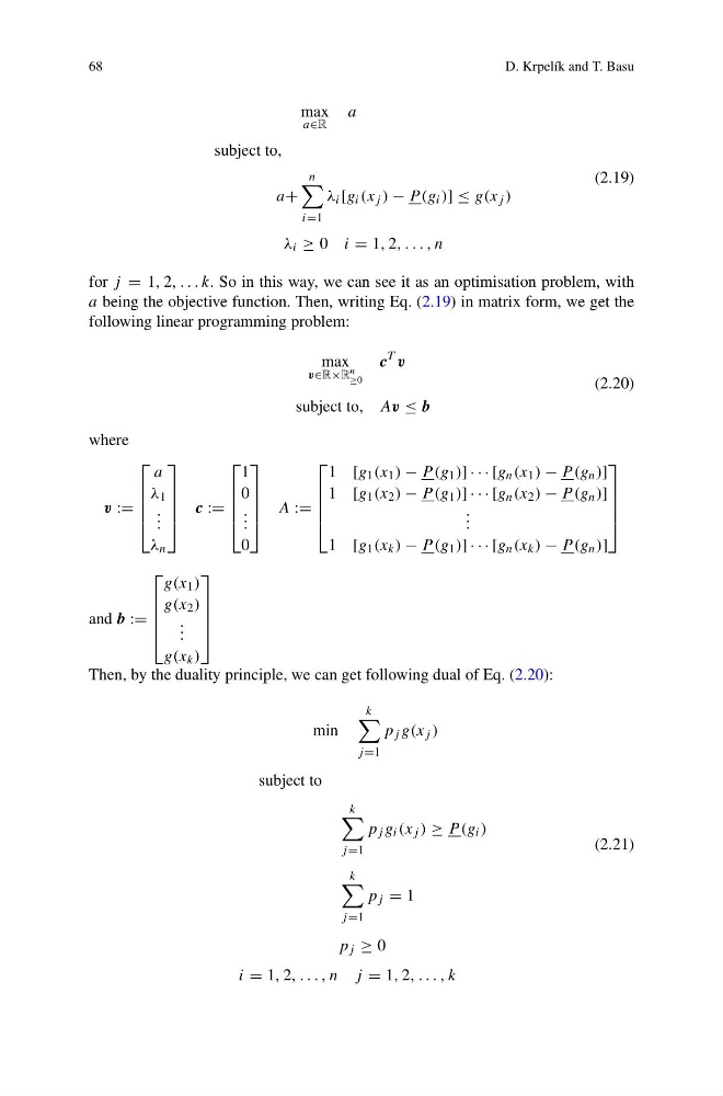
for j = 1, 2, . . . k. So in this way, we can see it as an optimisation problem, with
a being the objective function. Then, writing Eq. (2.19) in matrix form, we get the
following linear programming problem:
max
v∈R×R n
≥0
c
T v
subject to, Av ≤ b
(2.20)
where
v :=
⎡
⎢
⎢
⎢
⎣
a
λ 1
. . .
λ n
⎤
⎥
⎥
⎥
⎦
c :=
⎡
⎢
⎢
⎢
⎣
1
0
. . .
0
⎤
⎥
⎥
⎥
⎦
A :=
⎡
⎢
⎢
⎢
⎣
1 [g 1 (x 1 ) − P (g 1 )] · · · [g n (x 1 ) − P (g n )]
1 [g 1 (x 2 ) − P (g 1 )] · · · [g n (x 2 ) − P (g n )]
. . .
1 [g 1 (x k ) − P (g 1 )] · · · [g n (x k ) − P (g n )]
⎤
⎥
⎥
⎥
⎦
and b :=
⎡
⎢
⎢
⎢
⎣
g(x 1 )
g(x 2 )
. . .
g(x k )
⎤
⎥
⎥
⎥
⎦
Then, by the duality principle, we can get following dual of Eq. (2.20):
min
k
j =1
p j g(x j )
subject to
k
j =1
p j g i (x j ) ≥ P (g i )
k
j =1
p j = 1
p j ≥ 0
i = 1, 2, . . . , n j = 1, 2, . . . , k
(2.21)
D. Krpelík and T. Basu
max
a∈R
a
subject to,
a+
n
i=1
λ i [g i (x j ) − P (g i )] ≤ g(x j )
λ i ≥ 0 i = 1, 2, . . . , n
(2.19)
for j = 1, 2, . . . k. So in this way, we can see it as an optimisation problem, with
a being the objective function. Then, writing Eq. (2.19) in matrix form, we get the
following linear programming problem:
max
v∈R×R n
≥0
c
T v
subject to, Av ≤ b
(2.20)
where
v :=
⎡
⎢
⎢
⎢
⎣
a
λ 1
. . .
λ n
⎤
⎥
⎥
⎥
⎦
c :=
⎡
⎢
⎢
⎢
⎣
1
0
. . .
0
⎤
⎥
⎥
⎥
⎦
A :=
⎡
⎢
⎢
⎢
⎣
1 [g 1 (x 1 ) − P (g 1 )] · · · [g n (x 1 ) − P (g n )]
1 [g 1 (x 2 ) − P (g 1 )] · · · [g n (x 2 ) − P (g n )]
. . .
1 [g 1 (x k ) − P (g 1 )] · · · [g n (x k ) − P (g n )]
⎤
⎥
⎥
⎥
⎦
and b :=
⎡
⎢
⎢
⎢
⎣
g(x 1 )
g(x 2 )
. . .
g(x k )
⎤
⎥
⎥
⎥
⎦
Then, by the duality principle, we can get following dual of Eq. (2.20):
min
k
j =1
p j g(x j )
subject to
k
j =1
p j g i (x j ) ≥ P (g i )
k
j =1
p j = 1
p j ≥ 0
i = 1, 2, . . . , n j = 1, 2, . . . , k
(2.21)