

2 Introduction to Imprecise Probabilities
61
the tightest bounds for the respective probabilities over all the possible probability
distributions compliant to these assumptions. If the population mean and variance
are unknown, Saw [36] has proposed a variant of the Chebyshev’s inequality based
on their sample estimates.
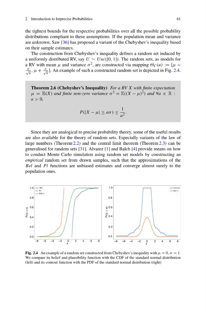
The construction from Chebyshev’s inequality defines a random set induced by
a uniformly distributed RV, say U ∼ Uni([0, 1]). The random sets, as models for
a RV with mean μ and variance σ 2 , are constructed via mapping Θ C (u) := [μ −
σ
√
u
, μ +
σ
√
u
]. An example of such a constructed random set is depicted in Fig. 2.4.
Theorem 2.6 (Chebyshev’s Inequality) For a RV X with finite expectation
μ = E(X) and finite non-zero variance σ 2 = E((X − μ) 2 ) and ∀a ∈ R :
a > 0,
P (|X − μ| ≥ aσ ) ≤
1
a 2 .
Since they are analogical to precise probability theory, some of the useful results
are also available for the theory of random sets. Especially variants of the law of
large numbers (Theorem 2.2) and the central limit theorem (Theorem 2.3) can be
generalised for random sets [31]. Alvarez [1] and Balch [4] provide means on how
to conduct Monte Carlo simulation using random set models by constructing an
empirical random set from drawn samples, such that the approximations of the
Bel and P l functions are unbiased estimates and converge almost surely to the
population ones.
1.0
0.8
0.6
0.4
0.2
0.0
–8
–6
–4
–2
0
2
4
6
8
x
Pr(x < x)
BEL
PL
N(0,1)
–8
–6
–4
–2
0
2
4
6
8
1.0
0.8
0.6
0.4
0.2
0.0
x
Pr(x
ѳ)
Contour
N(0,1)
Fig. 2.4 An example of a random set constructed from Chebyshev’s inequality with μ = 0, σ = 1.
We compare its belief and plausibility function with the CDF of the standard normal distribution
(left) and its contour function with the PDF of the standard normal distribution (right)
61
the tightest bounds for the respective probabilities over all the possible probability
distributions compliant to these assumptions. If the population mean and variance
are unknown, Saw [36] has proposed a variant of the Chebyshev’s inequality based
on their sample estimates.
The construction from Chebyshev’s inequality defines a random set induced by
a uniformly distributed RV, say U ∼ Uni([0, 1]). The random sets, as models for
a RV with mean μ and variance σ 2 , are constructed via mapping Θ C (u) := [μ −
σ
√
u
, μ +
σ
√
u
]. An example of such a constructed random set is depicted in Fig. 2.4.
Theorem 2.6 (Chebyshev’s Inequality) For a RV X with finite expectation
μ = E(X) and finite non-zero variance σ 2 = E((X − μ) 2 ) and ∀a ∈ R :
a > 0,
P (|X − μ| ≥ aσ ) ≤
1
a 2 .
Since they are analogical to precise probability theory, some of the useful results
are also available for the theory of random sets. Especially variants of the law of
large numbers (Theorem 2.2) and the central limit theorem (Theorem 2.3) can be
generalised for random sets [31]. Alvarez [1] and Balch [4] provide means on how
to conduct Monte Carlo simulation using random set models by constructing an
empirical random set from drawn samples, such that the approximations of the
Bel and P l functions are unbiased estimates and converge almost surely to the
population ones.
1.0
0.8
0.6
0.4
0.2
0.0
–8
–6
–4
–2
0
2
4
6
8
x
Pr(x < x)
BEL
PL
N(0,1)
–8
–6
–4
–2
0
2
4
6
8
1.0
0.8
0.6
0.4
0.2
0.0
x
Pr(x
ѳ)
Contour
N(0,1)
Fig. 2.4 An example of a random set constructed from Chebyshev’s inequality with μ = 0, σ = 1.
We compare its belief and plausibility function with the CDF of the standard normal distribution
(left) and its contour function with the PDF of the standard normal distribution (right)