

54
D. Krpelík and T. Basu
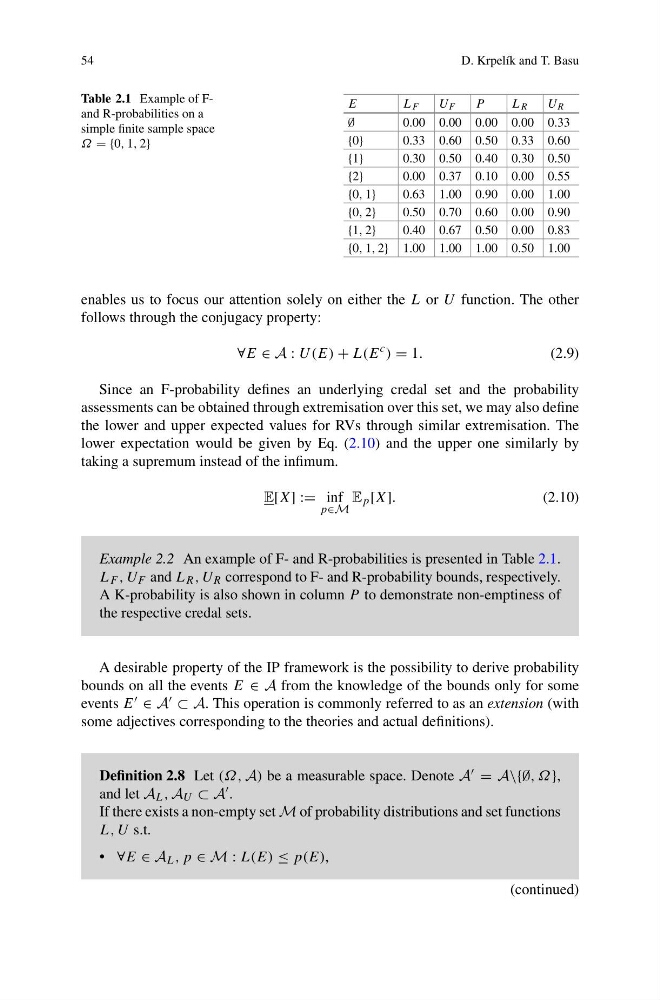
Table 2.1 Example of Fand R-probabilities on a
simple finite sample space
Ω = {0, 1, 2}
E
L F
U F
P
L R
U R
∅
0.00 0.00 0.00 0.00 0.33
{0}
0.33 0.60 0.50 0.33 0.60
{1}
0.30 0.50 0.40 0.30 0.50
{2}
0.00 0.37 0.10 0.00 0.55
{0, 1}
0.63 1.00 0.90 0.00 1.00
{0, 2}
0.50 0.70 0.60 0.00 0.90
{1, 2}
0.40 0.67 0.50 0.00 0.83
{0, 1, 2} 1.00 1.00 1.00 0.50 1.00
enables us to focus our attention solely on either the L or U function. The other
follows through the conjugacy property:
∀E ∈ A : U(E) + L(E
c ) = 1.
(2.9)
Since an F-probability defines an underlying credal set and the probability
assessments can be obtained through extremisation over this set, we may also define
the lower and upper expected values for RVs through similar extremisation. The
lower expectation would be given by Eq. (2.10) and the upper one similarly by
taking a supremum instead of the infimum.
E[X] := inf
p∈M
E p [X].
(2.10)
Example 2.2 An example of F- and R-probabilities is presented in Table 2.1.
L F , U F and L R , U R correspond to F- and R-probability bounds, respectively.
A K-probability is also shown in column P to demonstrate non-emptiness of
the respective credal sets.
A desirable property of the IP framework is the possibility to derive probability
bounds on all the events E ∈ A from the knowledge of the bounds only for some
events E ∈ A ⊂ A. This operation is commonly referred to as an extension (with
some adjectives corresponding to the theories and actual definitions).
Definition 2.8 Let (Ω, A) be a measurable space. Denote A = A\{∅, Ω},
and let A L , A U ⊂ A .
If there exists a non-empty set M of probability distributions and set functions
L, U s.t.
• ∀E ∈ A L , p ∈ M : L(E) ≤ p(E),
(continued)
D. Krpelík and T. Basu
Table 2.1 Example of Fand R-probabilities on a
simple finite sample space
Ω = {0, 1, 2}
E
L F
U F
P
L R
U R
∅
0.00 0.00 0.00 0.00 0.33
{0}
0.33 0.60 0.50 0.33 0.60
{1}
0.30 0.50 0.40 0.30 0.50
{2}
0.00 0.37 0.10 0.00 0.55
{0, 1}
0.63 1.00 0.90 0.00 1.00
{0, 2}
0.50 0.70 0.60 0.00 0.90
{1, 2}
0.40 0.67 0.50 0.00 0.83
{0, 1, 2} 1.00 1.00 1.00 0.50 1.00
enables us to focus our attention solely on either the L or U function. The other
follows through the conjugacy property:
∀E ∈ A : U(E) + L(E
c ) = 1.
(2.9)
Since an F-probability defines an underlying credal set and the probability
assessments can be obtained through extremisation over this set, we may also define
the lower and upper expected values for RVs through similar extremisation. The
lower expectation would be given by Eq. (2.10) and the upper one similarly by
taking a supremum instead of the infimum.
E[X] := inf
p∈M
E p [X].
(2.10)
Example 2.2 An example of F- and R-probabilities is presented in Table 2.1.
L F , U F and L R , U R correspond to F- and R-probability bounds, respectively.
A K-probability is also shown in column P to demonstrate non-emptiness of
the respective credal sets.
A desirable property of the IP framework is the possibility to derive probability
bounds on all the events E ∈ A from the knowledge of the bounds only for some
events E ∈ A ⊂ A. This operation is commonly referred to as an extension (with
some adjectives corresponding to the theories and actual definitions).
Definition 2.8 Let (Ω, A) be a measurable space. Denote A = A\{∅, Ω},
and let A L , A U ⊂ A .
If there exists a non-empty set M of probability distributions and set functions
L, U s.t.
• ∀E ∈ A L , p ∈ M : L(E) ≤ p(E),
(continued)