

2 Introduction to Imprecise Probabilities
51
I E (ω) :=
1, ω ∈ E,
0, ω /
∈ E,
P (E) = E(I E ).
(2.8)
The prevision terminology was also adapted in the lower prevision theory.
An interesting feature, that both Whittle and de Finetti have presented, is the
possibility to extend our partial knowledge to other RVs. Given a set of known
expectations for RVs K ⊂ L(Ω), we can derive bounds for the expectation of
another RV Y /
∈ K. The procedure is called simply an extension.
To do this, we can use corollaries of the expectation axioms. Given two RVs
(mappings from the sample space) s.t. ∀ω ∈ Ω : X(ω) ≤ Y (ω), we can derive, due
to the linearity and positivity of the expectation functional, that E(X) ≤ E(Y ).
Therefore, if we already know the expectations E(X n ) of several RVs X n ,
we trivially know the expectation of their arbitrary countable linear combination
Z =
a i X i , which is E(Z) =
a i E(X i ).
For an arbitrary RV Y , we can obtain the lower bound on its expectation by taking
the supremum over all the RVs in the span of X 1 , . . . , X n , which are strictly lower
than Y . Similarly for the upper bound.
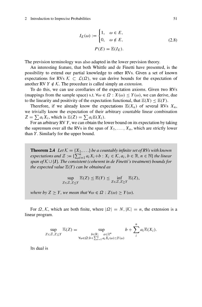
Theorem 2.4 Let K = {X 1 , . . .} be a countably infinite set of RVs with known
expectations and Z := {
n
i=1 a i X i +b : X i ∈ K, a i , b ∈ R, n ∈ N} the linear
span of K ∪ {1}. The consistent (coherent in de Finetti’s treatment) bounds for
the expected value E(Y ) can be obtained as
sup
Z∈Z,Z≤Y
E(Z) ≤ E(Y ) ≤
inf
Z∈Z,Z≥Y
E(Z),
where by Z ≥ Y , we mean that ∀ω ∈ Ω : Z(ω) ≥ Y (ω).
For Ω, K, which are both finite, where |Ω| = N, |K| = n, the extension is a
linear program.
sup
Z∈Z,Z≤Y
E(Z) =
sup
b∈R; a∈R n
∀ω∈Ω:b+
n
i=1 a i X i (ω)≤Y (ω)
b +
n
i
a i E(X i ).
Its dual is
51
I E (ω) :=
1, ω ∈ E,
0, ω /
∈ E,
P (E) = E(I E ).
(2.8)
The prevision terminology was also adapted in the lower prevision theory.
An interesting feature, that both Whittle and de Finetti have presented, is the
possibility to extend our partial knowledge to other RVs. Given a set of known
expectations for RVs K ⊂ L(Ω), we can derive bounds for the expectation of
another RV Y /
∈ K. The procedure is called simply an extension.
To do this, we can use corollaries of the expectation axioms. Given two RVs
(mappings from the sample space) s.t. ∀ω ∈ Ω : X(ω) ≤ Y (ω), we can derive, due
to the linearity and positivity of the expectation functional, that E(X) ≤ E(Y ).
Therefore, if we already know the expectations E(X n ) of several RVs X n ,
we trivially know the expectation of their arbitrary countable linear combination
Z =
a i X i , which is E(Z) =
a i E(X i ).
For an arbitrary RV Y , we can obtain the lower bound on its expectation by taking
the supremum over all the RVs in the span of X 1 , . . . , X n , which are strictly lower
than Y . Similarly for the upper bound.
Theorem 2.4 Let K = {X 1 , . . .} be a countably infinite set of RVs with known
expectations and Z := {
n
i=1 a i X i +b : X i ∈ K, a i , b ∈ R, n ∈ N} the linear
span of K ∪ {1}. The consistent (coherent in de Finetti’s treatment) bounds for
the expected value E(Y ) can be obtained as
sup
Z∈Z,Z≤Y
E(Z) ≤ E(Y ) ≤
inf
Z∈Z,Z≥Y
E(Z),
where by Z ≥ Y , we mean that ∀ω ∈ Ω : Z(ω) ≥ Y (ω).
For Ω, K, which are both finite, where |Ω| = N, |K| = n, the extension is a
linear program.
sup
Z∈Z,Z≤Y
E(Z) =
sup
b∈R; a∈R n
∀ω∈Ω:b+
n
i=1 a i X i (ω)≤Y (ω)
b +
n
i
a i E(X i ).
Its dual is