562
G. Filippi and M. Vasile
Algorithm 2 Decomposition
1: Initialise
2: Uncoupled vectors u u = [u 1 , u 2 , . . . , u i , . . . , u mu ]
3: Coupled vectors u c = [u 12 , u 13 , . . . , u ij , . . . , u mc ]
4: for a given design d do
5:
Compute ( d, u u , u c ) = arg max F ( d, u u , u c )
6:
for all u ij ∈ u c do
7:
for all Focal Elements θ k,ij ⊆ Θ ij do
8:
F k,ij = max u ij ∈θ k,ij F ( d, u u , u ij )
9:
u k,ij = argmax u ij ∈θ k,ij F
10:
Evaluate bpa(θ k,ij )
11:
Evaluate partial Belief curve Bel(F (u ij ) ≤ ν)
12:
end for
13:
for number of samples do
14:
Evaluate ΔBel q , u k,ij and
F k,ij
15:
end for
16:
end for
17:
for all the combinations of samples do
18:
for all u i ∈ u u do
19:
for all Focal Elements θ k,i ⊆ Θ i do
20:
Run
F max,k,i = max θ k,i F ( d, u c , u i )
21:
Evaluate bpa(θ k,i )
22:
end for
23:
end for
24:
for all the combinations of Focal Elements
θ t ∈ Θ 1 × Θ 2 × . . . × Θ mu do
25:
Evaluate F max,k ≤ ν
26:
Evaluate bpa k
27:
end for
28:
Evaluate the Belief for this sample by constructing collection Γ ν
29:
end for
30:
Add up all belief values for all samples
31: end for
We can then compute the partial belief associated only to the coupled variables with
index ij :
Bel(F (u ij ) < ν) =
θ k,ij | max u ij ∈θ k,ij F (u ij )≤ν
bpa(θ k,ij )
(17.54)
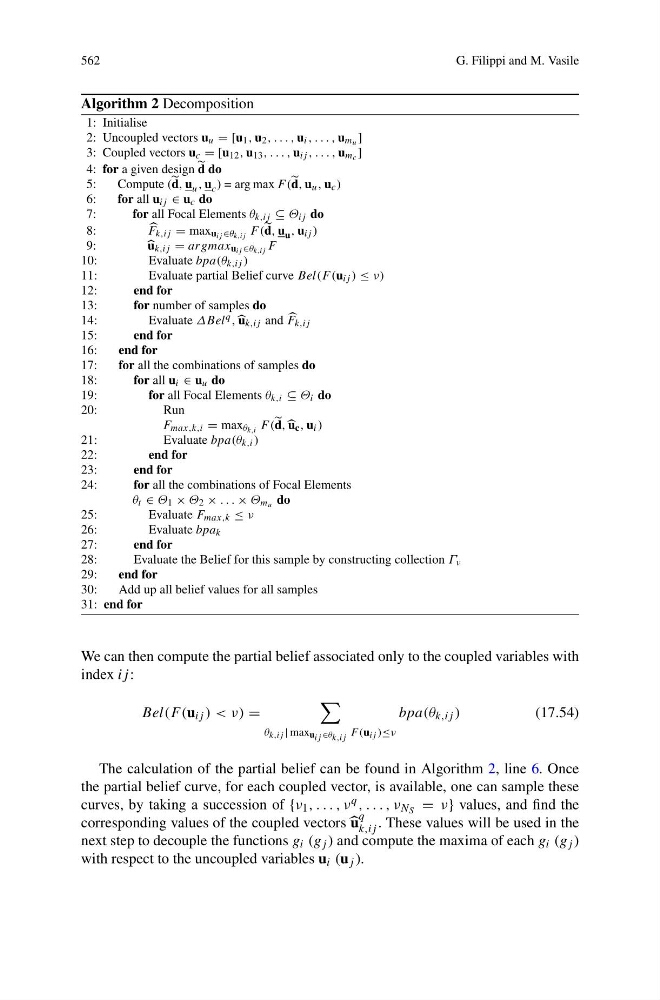
The calculation of the partial belief can be found in Algorithm 2, line 6. Once
the partial belief curve, for each coupled vector, is available, one can sample these
curves, by taking a succession of {ν 1 , . . . , ν q , . . . , ν N S = ν} values, and find the
corresponding values of the coupled vectors u
q
k,ij . These values will be used in the
next step to decouple the functions g i (g j ) and compute the maxima of each g i (g j )
with respect to the uncoupled variables u i (u j ).