

560
G. Filippi and M. Vasile
node i is characterised by the value function g i and exchanges information with
node j via the exchange function h ij . Following the definition of the design vector
d and uncertain vector u introduced in the previous sections, one can define the total
value of the network as:
f (d, u) =
N
i=1
g i (d, u i , h i (d, u i , u ij ))
(17.46)
where h i (d, u i , u ij ) is the vector of scalar functions h ij (d, u i , u ij ), j ∈ J i and J i is
the set of indexes of nodes connected to the i-th node; u i are the uncertain variables
of sub-system i not affecting any other sub-systems and u ij are the uncertain
variables affecting both sub-systems i and j . Please note that accordingly to our
notation u ij = u ji .
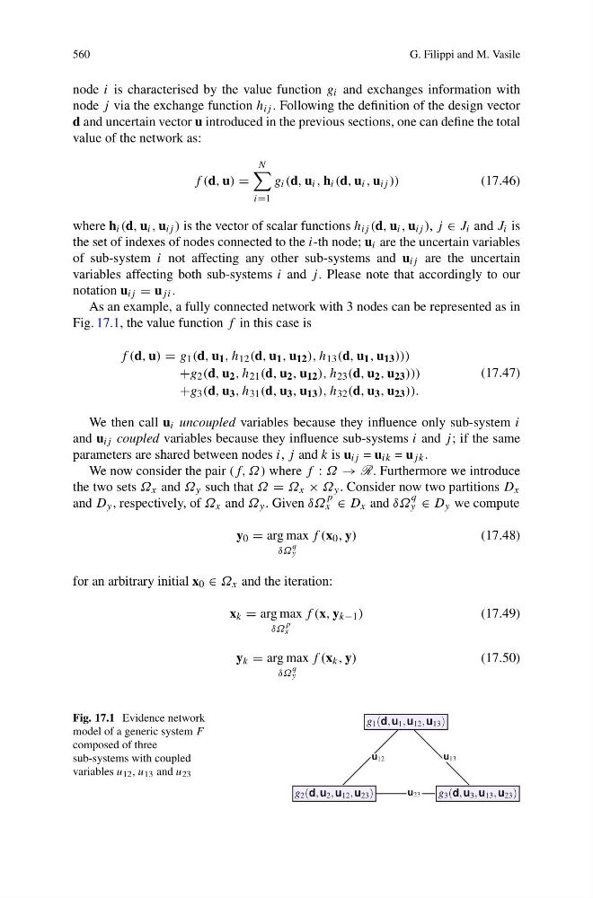
As an example, a fully connected network with 3 nodes can be represented as in
Fig. 17.1, the value function f in this case is
f (d, u) = g 1 (d, u 1 , h 12 (d, u 1 , u 12 ), h 13 (d, u 1 , u 13 )))
+g 2 (d, u 2 , h 21 (d, u 2 , u 12 ), h 23 (d, u 2 , u 23 )))
+g 3 (d, u 3 , h 31 (d, u 3 , u 13 ), h 32 (d, u 3 , u 23 )).
(17.47)
We then call u i uncoupled variables because they influence only sub-system i
and u ij coupled variables because they influence sub-systems i and j ; if the same
parameters are shared between nodes i, j and k is u ij = u ik = u jk .
We now consider the pair (f, Ω) where f : Ω → R. Furthermore we introduce
the two sets Ω x and Ω y such that Ω = Ω x × Ω y . Consider now two partitions D x
and D y , respectively, of Ω x and Ω y . Given δΩ
p
x ∈ D x and δΩ
q
y ∈ D y we compute
y 0 = arg max
δΩ
q
y
f (x 0 , y)
(17.48)
for an arbitrary initial x 0 ∈ Ω x and the iteration:
x k = arg max
δΩ
p
x
f (x, y k−1 )
(17.49)
y k = arg max
δΩ
q
y
f (x k , y)
(17.50)
Fig. 17.1 Evidence network
model of a generic system F
composed of three
sub-systems with coupled
variables u 12 , u 13 and u 23
g 1 (d, u 1 , u 12 , u 13 )
g 2 (d, u 2 , u 12 , u 23 )
g 3 (d, u 3 , u 13 , u 23 )
u 12
u 13
u 23