

13 Risk Measures in the Context of Robust and Reliability Based Optimization
423
⎧
⎪ ⎪ ⎪ ⎪ ⎪ ⎨
⎪ ⎪ ⎪ ⎪ ⎪ ⎩
c l = 0.5
t/c = 0.12
XT R LOW ≤ 0.95c
T EA ≥ 13 ◦
LER ≥ 0.007c
(13.27)
Hence, the robust optimization problem is formulated as:
min
z∈Z⊆R n
CV aR(Q)
(13.28)
with
Q = c d + p
+ (T EA, 13
◦ ) + p
+ (LER, 0.007c)
(13.29)
In this case the constraints regarding the leading edge radius and the training edge
angle are treated as quadratic penalties:
p
+ (x, y) =
0
i fx ≥ y
(x − y) 2 if x < y
(13.30)
Instead, the constraints on the c l and on the thickness do not appear because they
are automatically satisfied by the computation procedure by changing the angle of
attack and by re-scaling the airfoil thickness to the assigned value.
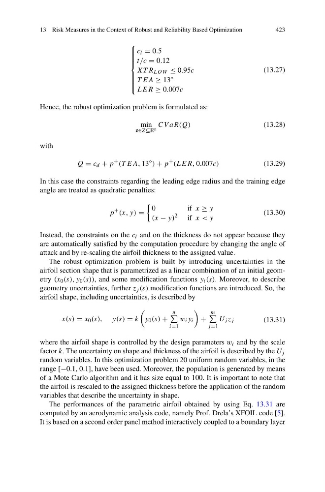
The robust optimization problem is built by introducing uncertainties in the
airfoil section shape that is parametrized as a linear combination of an initial geometry (x 0 (s), y 0 (s)), and some modification functions y i (s). Moreover, to describe
geometry uncertainties, further z j (s) modification functions are introduced. So, the
airfoil shape, including uncertainties, is described by
x(s) = x 0 (s), y(s) = k
y 0 (s) +
n
i=1
w i y i
+
m
j =1
U j z j
(13.31)
where the airfoil shape is controlled by the design parameters w i and by the scale
factor k. The uncertainty on shape and thickness of the airfoil is described by the U j
random variables. In this optimization problem 20 uniform random variables, in the
range [−0.1, 0.1], have been used. Moreover, the population is generated by means
of a Mote Carlo algorithm and it has size equal to 100. It is important to note that
the airfoil is rescaled to the assigned thickness before the application of the random
variables that describe the uncertainty in shape.
The performances of the parametric airfoil obtained by using Eq. 13.31 are
computed by an aerodynamic analysis code, namely Prof. Drela’s XFOIL code [5].
It is based on a second order panel method interactively coupled to a boundary layer
423
⎧
⎪ ⎪ ⎪ ⎪ ⎪ ⎨
⎪ ⎪ ⎪ ⎪ ⎪ ⎩
c l = 0.5
t/c = 0.12
XT R LOW ≤ 0.95c
T EA ≥ 13 ◦
LER ≥ 0.007c
(13.27)
Hence, the robust optimization problem is formulated as:
min
z∈Z⊆R n
CV aR(Q)
(13.28)
with
Q = c d + p
+ (T EA, 13
◦ ) + p
+ (LER, 0.007c)
(13.29)
In this case the constraints regarding the leading edge radius and the training edge
angle are treated as quadratic penalties:
p
+ (x, y) =
0
i fx ≥ y
(x − y) 2 if x < y
(13.30)
Instead, the constraints on the c l and on the thickness do not appear because they
are automatically satisfied by the computation procedure by changing the angle of
attack and by re-scaling the airfoil thickness to the assigned value.
The robust optimization problem is built by introducing uncertainties in the
airfoil section shape that is parametrized as a linear combination of an initial geometry (x 0 (s), y 0 (s)), and some modification functions y i (s). Moreover, to describe
geometry uncertainties, further z j (s) modification functions are introduced. So, the
airfoil shape, including uncertainties, is described by
x(s) = x 0 (s), y(s) = k
y 0 (s) +
n
i=1
w i y i
+
m
j =1
U j z j
(13.31)
where the airfoil shape is controlled by the design parameters w i and by the scale
factor k. The uncertainty on shape and thickness of the airfoil is described by the U j
random variables. In this optimization problem 20 uniform random variables, in the
range [−0.1, 0.1], have been used. Moreover, the population is generated by means
of a Mote Carlo algorithm and it has size equal to 100. It is important to note that
the airfoil is rescaled to the assigned thickness before the application of the random
variables that describe the uncertainty in shape.
The performances of the parametric airfoil obtained by using Eq. 13.31 are
computed by an aerodynamic analysis code, namely Prof. Drela’s XFOIL code [5].
It is based on a second order panel method interactively coupled to a boundary layer