

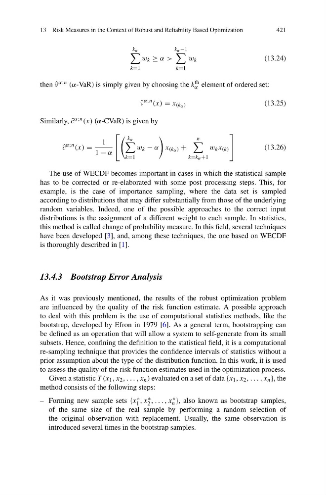
13 Risk Measures in the Context of Robust and Reliability Based Optimization
421
k α
k=1
w k ≥ α >
k α −1
k=1
w k
(13.24)
then ˆ
ν α;n (α-VaR) is simply given by choosing the k th
α element of ordered set:
ˆ
ν
α;n (x) = x (k α )
(13.25)
Similarly, ˆ
c α;n (x) (α-CVaR) is given by
ˆ
c
α;n (x) =
1
1 − α
⎡
⎣
k α
k=1
w k − α
x (k α ) +
n
k=k α +1
w k x (k)
⎤
⎦
(13.26)
The use of WECDF becomes important in cases in which the statistical sample
has to be corrected or re-elaborated with some post processing steps. This, for
example, is the case of importance sampling, where the data set is sampled
according to distributions that may differ substantially from those of the underlying
random variables. Indeed, one of the possible approaches to the correct input
distributions is the assignment of a different weight to each sample. In statistics,
this method is called change of probability measure. In this field, several techniques
have been developed [3], and, among these techniques, the one based on WECDF
is thoroughly described in [1].
13.4.3 Bootstrap Error Analysis
As it was previously mentioned, the results of the robust optimization problem
are influenced by the quality of the risk function estimate. A possible approach
to deal with this problem is the use of computational statistics methods, like the
bootstrap, developed by Efron in 1979 [6]. As a general term, bootstrapping can
be defined as an operation that will allow a system to self-generate from its small
subsets. Hence, confining the definition to the statistical field, it is a computational
re-sampling technique that provides the confidence intervals of statistics without a
prior assumption about the type of the distribution function. In this work, it is used
to assess the quality of the risk function estimates used in the optimization process.
Given a statistic T (x 1 , x 2 , . . . , x n ) evaluated on a set of data {x 1 , x 2 , . . . , x n }, the
method consists of the following steps:
– Forming new sample sets {x ∗
1 , x ∗
2 , . . . , x ∗
n }, also known as bootstrap samples,
of the same size of the real sample by performing a random selection of
the original observation with replacement. Usually, the same observation is
introduced several times in the bootstrap samples.
421
k α
k=1
w k ≥ α >
k α −1
k=1
w k
(13.24)
then ˆ
ν α;n (α-VaR) is simply given by choosing the k th
α element of ordered set:
ˆ
ν
α;n (x) = x (k α )
(13.25)
Similarly, ˆ
c α;n (x) (α-CVaR) is given by
ˆ
c
α;n (x) =
1
1 − α
⎡
⎣
k α
k=1
w k − α
x (k α ) +
n
k=k α +1
w k x (k)
⎤
⎦
(13.26)
The use of WECDF becomes important in cases in which the statistical sample
has to be corrected or re-elaborated with some post processing steps. This, for
example, is the case of importance sampling, where the data set is sampled
according to distributions that may differ substantially from those of the underlying
random variables. Indeed, one of the possible approaches to the correct input
distributions is the assignment of a different weight to each sample. In statistics,
this method is called change of probability measure. In this field, several techniques
have been developed [3], and, among these techniques, the one based on WECDF
is thoroughly described in [1].
13.4.3 Bootstrap Error Analysis
As it was previously mentioned, the results of the robust optimization problem
are influenced by the quality of the risk function estimate. A possible approach
to deal with this problem is the use of computational statistics methods, like the
bootstrap, developed by Efron in 1979 [6]. As a general term, bootstrapping can
be defined as an operation that will allow a system to self-generate from its small
subsets. Hence, confining the definition to the statistical field, it is a computational
re-sampling technique that provides the confidence intervals of statistics without a
prior assumption about the type of the distribution function. In this work, it is used
to assess the quality of the risk function estimates used in the optimization process.
Given a statistic T (x 1 , x 2 , . . . , x n ) evaluated on a set of data {x 1 , x 2 , . . . , x n }, the
method consists of the following steps:
– Forming new sample sets {x ∗
1 , x ∗
2 , . . . , x ∗
n }, also known as bootstrap samples,
of the same size of the real sample by performing a random selection of
the original observation with replacement. Usually, the same observation is
introduced several times in the bootstrap samples.