

12 Response Surface Methodology
399
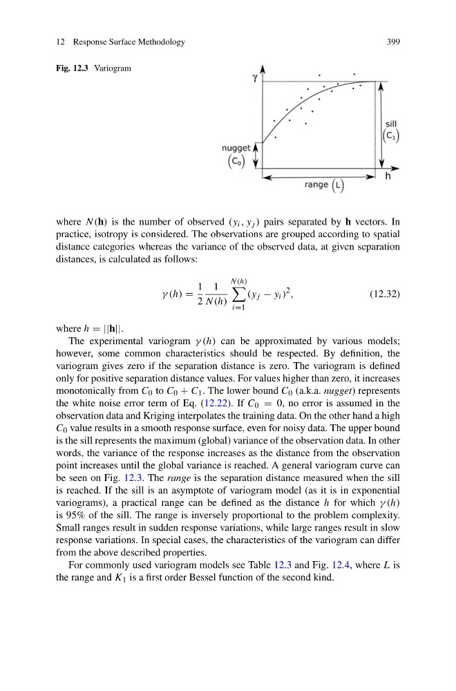
Fig. 12.3 Variogram
where N(h) is the number of observed (y i , y j ) pairs separated by h vectors. In
practice, isotropy is considered. The observations are grouped according to spatial
distance categories whereas the variance of the observed data, at given separation
distances, is calculated as follows:
γ (h) =
1
2
1
N(h)
N(h)
i=1
(y j − y i )
2 ,
(12.32)
where h = ||h||.
The experimental variogram γ (h) can be approximated by various models;
however, some common characteristics should be respected. By definition, the
variogram gives zero if the separation distance is zero. The variogram is defined
only for positive separation distance values. For values higher than zero, it increases
monotonically from C 0 to C 0 + C 1 . The lower bound C 0 (a.k.a. nugget) represents
the white noise error term of Eq. (12.22). If C 0 = 0, no error is assumed in the
observation data and Kriging interpolates the training data. On the other hand a high
C 0 value results in a smooth response surface, even for noisy data. The upper bound
is the sill represents the maximum (global) variance of the observation data. In other
words, the variance of the response increases as the distance from the observation
point increases until the global variance is reached. A general variogram curve can
be seen on Fig. 12.3. The range is the separation distance measured when the sill
is reached. If the sill is an asymptote of variogram model (as it is in exponential
variograms), a practical range can be defined as the distance h for which γ (h)
is 95% of the sill. The range is inversely proportional to the problem complexity.
Small ranges result in sudden response variations, while large ranges result in slow
response variations. In special cases, the characteristics of the variogram can differ
from the above described properties.
For commonly used variogram models see Table 12.3 and Fig. 12.4, where L is
the range and K 1 is a first order Bessel function of the second kind.
399
Fig. 12.3 Variogram
where N(h) is the number of observed (y i , y j ) pairs separated by h vectors. In
practice, isotropy is considered. The observations are grouped according to spatial
distance categories whereas the variance of the observed data, at given separation
distances, is calculated as follows:
γ (h) =
1
2
1
N(h)
N(h)
i=1
(y j − y i )
2 ,
(12.32)
where h = ||h||.
The experimental variogram γ (h) can be approximated by various models;
however, some common characteristics should be respected. By definition, the
variogram gives zero if the separation distance is zero. The variogram is defined
only for positive separation distance values. For values higher than zero, it increases
monotonically from C 0 to C 0 + C 1 . The lower bound C 0 (a.k.a. nugget) represents
the white noise error term of Eq. (12.22). If C 0 = 0, no error is assumed in the
observation data and Kriging interpolates the training data. On the other hand a high
C 0 value results in a smooth response surface, even for noisy data. The upper bound
is the sill represents the maximum (global) variance of the observation data. In other
words, the variance of the response increases as the distance from the observation
point increases until the global variance is reached. A general variogram curve can
be seen on Fig. 12.3. The range is the separation distance measured when the sill
is reached. If the sill is an asymptote of variogram model (as it is in exponential
variograms), a practical range can be defined as the distance h for which γ (h)
is 95% of the sill. The range is inversely proportional to the problem complexity.
Small ranges result in sudden response variations, while large ranges result in slow
response variations. In special cases, the characteristics of the variogram can differ
from the above described properties.
For commonly used variogram models see Table 12.3 and Fig. 12.4, where L is
the range and K 1 is a first order Bessel function of the second kind.