

340
L. Gentile et al.
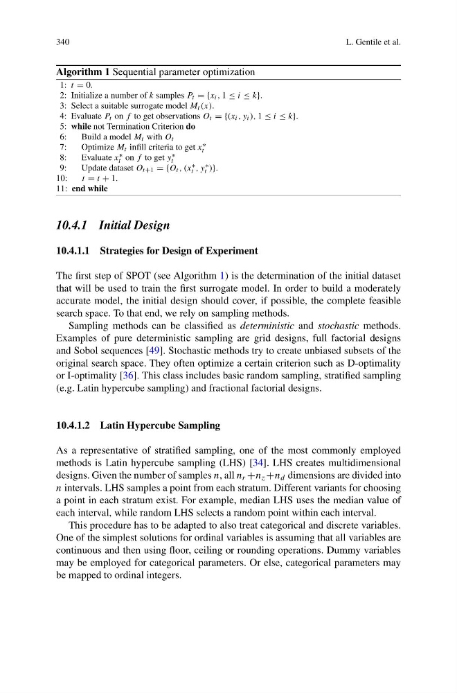
Algorithm 1 Sequential parameter optimization
1: t = 0.
2: Initialize a number of k samples P t = {x i , 1 ≤ i ≤ k}.
3: Select a suitable surrogate model M t (x).
4: Evaluate P t on f to get observations O t = {(x i , y i ), 1 ≤ i ≤ k}.
5: while not Termination Criterion do
6:
Build a model M t with O t
7:
Optimize M t infill criteria to get x ∗
t
8:
Evaluate x ∗
t on f to get y ∗
t
9:
Update dataset O t+1 = {O t , (x ∗
t , y ∗
t )}.
10:
t = t + 1.
11: end while
10.4.1 Initial Design
10.4.1.1 Strategies for Design of Experiment
The first step of SPOT (see Algorithm 1) is the determination of the initial dataset
that will be used to train the first surrogate model. In order to build a moderately
accurate model, the initial design should cover, if possible, the complete feasible
search space. To that end, we rely on sampling methods.
Sampling methods can be classified as deterministic and stochastic methods.
Examples of pure deterministic sampling are grid designs, full factorial designs
and Sobol sequences [49]. Stochastic methods try to create unbiased subsets of the
original search space. They often optimize a certain criterion such as D-optimality
or I-optimality [36]. This class includes basic random sampling, stratified sampling
(e.g. Latin hypercube sampling) and fractional factorial designs.
10.4.1.2 Latin Hypercube Sampling
As a representative of stratified sampling, one of the most commonly employed
methods is Latin hypercube sampling (LHS) [34]. LHS creates multidimensional
designs. Given the number of samples n, all n r +n z +n d dimensions are divided into
n intervals. LHS samples a point from each stratum. Different variants for choosing
a point in each stratum exist. For example, median LHS uses the median value of
each interval, while random LHS selects a random point within each interval.
This procedure has to be adapted to also treat categorical and discrete variables.
One of the simplest solutions for ordinal variables is assuming that all variables are
continuous and then using floor, ceiling or rounding operations. Dummy variables
may be employed for categorical parameters. Or else, categorical parameters may
be mapped to ordinal integers.
L. Gentile et al.
Algorithm 1 Sequential parameter optimization
1: t = 0.
2: Initialize a number of k samples P t = {x i , 1 ≤ i ≤ k}.
3: Select a suitable surrogate model M t (x).
4: Evaluate P t on f to get observations O t = {(x i , y i ), 1 ≤ i ≤ k}.
5: while not Termination Criterion do
6:
Build a model M t with O t
7:
Optimize M t infill criteria to get x ∗
t
8:
Evaluate x ∗
t on f to get y ∗
t
9:
Update dataset O t+1 = {O t , (x ∗
t , y ∗
t )}.
10:
t = t + 1.
11: end while
10.4.1 Initial Design
10.4.1.1 Strategies for Design of Experiment
The first step of SPOT (see Algorithm 1) is the determination of the initial dataset
that will be used to train the first surrogate model. In order to build a moderately
accurate model, the initial design should cover, if possible, the complete feasible
search space. To that end, we rely on sampling methods.
Sampling methods can be classified as deterministic and stochastic methods.
Examples of pure deterministic sampling are grid designs, full factorial designs
and Sobol sequences [49]. Stochastic methods try to create unbiased subsets of the
original search space. They often optimize a certain criterion such as D-optimality
or I-optimality [36]. This class includes basic random sampling, stratified sampling
(e.g. Latin hypercube sampling) and fractional factorial designs.
10.4.1.2 Latin Hypercube Sampling
As a representative of stratified sampling, one of the most commonly employed
methods is Latin hypercube sampling (LHS) [34]. LHS creates multidimensional
designs. Given the number of samples n, all n r +n z +n d dimensions are divided into
n intervals. LHS samples a point from each stratum. Different variants for choosing
a point in each stratum exist. For example, median LHS uses the median value of
each interval, while random LHS selects a random point within each interval.
This procedure has to be adapted to also treat categorical and discrete variables.
One of the simplest solutions for ordinal variables is assuming that all variables are
continuous and then using floor, ceiling or rounding operations. Dummy variables
may be employed for categorical parameters. Or else, categorical parameters may
be mapped to ordinal integers.