

318
M. Antoniou and P. Korošec
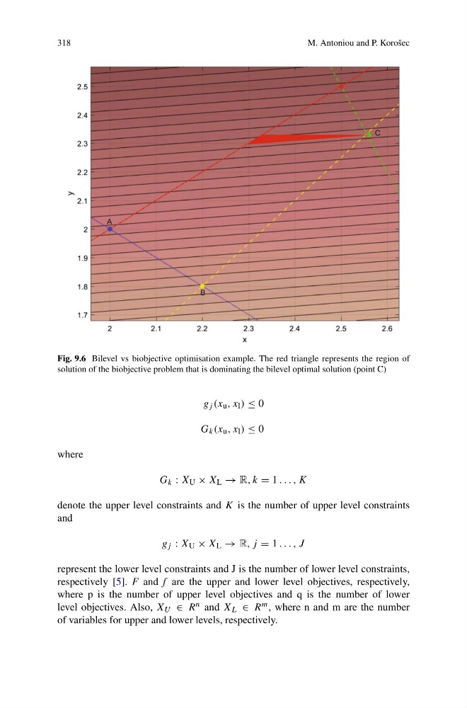
Fig. 9.6 Bilevel vs biobjective optimisation example. The red triangle represents the region of
solution of the biobjective problem that is dominating the bilevel optimal solution (point C)
g j (x u , x l ) ≤ 0
G k (x u , x l ) ≤ 0
where
G k : X U × X L → R, k = 1 . . . , K
denote the upper level constraints and K is the number of upper level constraints
and
g j : X U × X L → R, j = 1 . . . , J
represent the lower level constraints and J is the number of lower level constraints,
respectively [5]. F and f are the upper and lower level objectives, respectively,
where p is the number of upper level objectives and q is the number of lower
level objectives. Also, X U ∈ R n and X L ∈ R m , where n and m are the number
of variables for upper and lower levels, respectively.
M. Antoniou and P. Korošec
Fig. 9.6 Bilevel vs biobjective optimisation example. The red triangle represents the region of
solution of the biobjective problem that is dominating the bilevel optimal solution (point C)
g j (x u , x l ) ≤ 0
G k (x u , x l ) ≤ 0
where
G k : X U × X L → R, k = 1 . . . , K
denote the upper level constraints and K is the number of upper level constraints
and
g j : X U × X L → R, j = 1 . . . , J
represent the lower level constraints and J is the number of lower level constraints,
respectively [5]. F and f are the upper and lower level objectives, respectively,
where p is the number of upper level objectives and q is the number of lower
level objectives. Also, X U ∈ R n and X L ∈ R m , where n and m are the number
of variables for upper and lower levels, respectively.