

316
M. Antoniou and P. Korošec
2
2.1
2.2
2.3
2.4
2.5
2.6
x
1.8
1.9
2
2.1
2.2
2.3
2.4
2.5
y
Scatter plot of feasible decision variable space
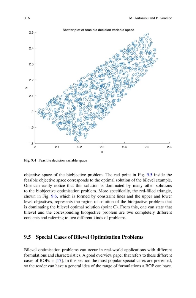
Fig. 9.4 Feasible decision variable space
objective space of the biobjective problem. The red point in Fig. 9.5 inside the
feasible objective space corresponds to the optimal solution of the bilevel example.
One can easily notice that this solution is dominated by many other solutions
to the biobjective optimisation problem. More specifically, the red-filled triangle,
shown in Fig. 9.6, which is formed by constraint lines and the upper and lower
level objectives, represents the region of solution of the biobjective problem that
is dominating the bilevel optimal solution (point C). From this, one can state that
bilevel and the corresponding biobjective problem are two completely different
concepts and referring to two different kinds of problems.
9.5 Special Cases of Bilevel Optimisation Problems
Bilevel optimisation problems can occur in real-world applications with different
formulations and characteristics. A good overview paper that refers to these different
cases of BOPs is [17]. In this section the most popular special cases are presented,
so the reader can have a general idea of the range of formulations a BOP can have.
M. Antoniou and P. Korošec
2
2.1
2.2
2.3
2.4
2.5
2.6
x
1.8
1.9
2
2.1
2.2
2.3
2.4
2.5
y
Scatter plot of feasible decision variable space
Fig. 9.4 Feasible decision variable space
objective space of the biobjective problem. The red point in Fig. 9.5 inside the
feasible objective space corresponds to the optimal solution of the bilevel example.
One can easily notice that this solution is dominated by many other solutions
to the biobjective optimisation problem. More specifically, the red-filled triangle,
shown in Fig. 9.6, which is formed by constraint lines and the upper and lower
level objectives, represents the region of solution of the biobjective problem that
is dominating the bilevel optimal solution (point C). From this, one can state that
bilevel and the corresponding biobjective problem are two completely different
concepts and referring to two different kinds of problems.
9.5 Special Cases of Bilevel Optimisation Problems
Bilevel optimisation problems can occur in real-world applications with different
formulations and characteristics. A good overview paper that refers to these different
cases of BOPs is [17]. In this section the most popular special cases are presented,
so the reader can have a general idea of the range of formulations a BOP can have.