

24
J. F. Reis et al.
1.6.2.2 Linear Regression
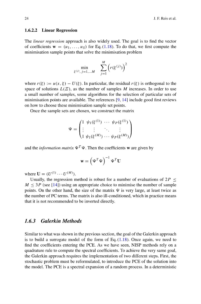
The linear regression approach is also widely used. The goal is to find the vector
of coefficients w = (u 1 , . . . , u S ) for Eq. (1.18). To do that, we first compute the
minimisation sample points that solve the minimisation problem
min
ξ (j ) , j=1,...M
M
j =1
r(ξ
(j ) )
2
where r(ξ ) := u(x, ξ ) − U(ξ). In particular, the residual r(ξ ) is orthogonal to the
space of solutions L(Ξ ), as the number of samples M increases. In order to use
a small number of samples, some algorithms for the selection of particular sets of
minimisation points are available. The references [9, 14] include good first reviews
on how to choose these minimisation sample set points.
Once the sample sets are chosen, we construct the matrix
=
⎛
⎜
⎝
1 ψ 1 (ξ (1) ) · · · ψ P (ξ (1) )
. . .
. . .
. . .
. . .
1 ψ 1 (ξ (M) ) · · · ψ P (ξ (M) )
⎞
⎟
⎠
and the information matrix T . Then the coefficients w are given by
w =
T
−1
T U
where U = (U (1) · · · U (M) ).
Usually, the regression method is robust for a number of evaluations of 2P ≤
M ≤ 3P (see [14]) using an appropriate choice to minimise the number of sample
points. On the other hand, the size of the matrix is very large, at least twice as
the number of PC terms. The matrix is also ill-conditioned, which in practice means
that it is not recommended to be inverted directly.
1.6.3 Galerkin Methods
Similar to what was shown in the previous section, the goal of the Galerkin approach
is to build a surrogate model of the form of Eq. (1.18). Once again, we need to
find the coefficients entering the PCE. As we have seen, NISP methods rely on a
quadrature rule to compute the spectral coefficients. To achieve the very same goal,
the Galerkin approach requires the implementation of two different steps. First, the
stochastic problem must be reformulated, to introduce the PCE of the solution into
the model. The PCE is a spectral expansion of a random process. In a deterministic
J. F. Reis et al.
1.6.2.2 Linear Regression
The linear regression approach is also widely used. The goal is to find the vector
of coefficients w = (u 1 , . . . , u S ) for Eq. (1.18). To do that, we first compute the
minimisation sample points that solve the minimisation problem
min
ξ (j ) , j=1,...M
M
j =1
r(ξ
(j ) )
2
where r(ξ ) := u(x, ξ ) − U(ξ). In particular, the residual r(ξ ) is orthogonal to the
space of solutions L(Ξ ), as the number of samples M increases. In order to use
a small number of samples, some algorithms for the selection of particular sets of
minimisation points are available. The references [9, 14] include good first reviews
on how to choose these minimisation sample set points.
Once the sample sets are chosen, we construct the matrix
=
⎛
⎜
⎝
1 ψ 1 (ξ (1) ) · · · ψ P (ξ (1) )
. . .
. . .
. . .
. . .
1 ψ 1 (ξ (M) ) · · · ψ P (ξ (M) )
⎞
⎟
⎠
and the information matrix T . Then the coefficients w are given by
w =
T
−1
T U
where U = (U (1) · · · U (M) ).
Usually, the regression method is robust for a number of evaluations of 2P ≤
M ≤ 3P (see [14]) using an appropriate choice to minimise the number of sample
points. On the other hand, the size of the matrix is very large, at least twice as
the number of PC terms. The matrix is also ill-conditioned, which in practice means
that it is not recommended to be inverted directly.
1.6.3 Galerkin Methods
Similar to what was shown in the previous section, the goal of the Galerkin approach
is to build a surrogate model of the form of Eq. (1.18). Once again, we need to
find the coefficients entering the PCE. As we have seen, NISP methods rely on a
quadrature rule to compute the spectral coefficients. To achieve the very same goal,
the Galerkin approach requires the implementation of two different steps. First, the
stochastic problem must be reformulated, to introduce the PCE of the solution into
the model. The PCE is a spectral expansion of a random process. In a deterministic