

6 Fundamentals of Filtering
209
δx 0 ∼ N δx 0 (ˆ x 0 − ¯
x 0 , P 0 ) .
(6.77)
This property on the covariance holds at any time P δx = P x because the reference
point ˆ
x is deterministic and fixed. The linearised system can be solved directly with
the Kalman filter.
There is freedom in the choice of the reference point ¯
x 0 , and the obvious choice is
¯
x 0 = ˆ
x 0 . In this case, from Eq. (6.77) and Eq.(6.33), it is straightforward to see that,
before any observation update, E{δx} =
δx = 0. This is a valuable characteristic as
the linearised model results accurate only for relatively small deviations. However,
when an observation comes in, the update step changes the best estimate to ˆ
x
+
k from
the reference value ¯
x k = ˆ
x
−
k . In particular, when the covariance matrix of the state
P
−
k is large, i.e. the estimate is not a proper measure of the distribution, the Kalman
gain is large, and therefore the update step will cause the new estimate to deviate
significantly from the reference state. In sequential filtering, the workaround is to relinearise the trajectory around the new best estimate ˆ
x
+
k after an observation update.
Indeed, if we assume that an observation is improving our knowledge of the state,
then it is natural to linearise around a point supposedly closer to the true state to
have smaller nonlinearity-induced errors. With this procedure, the expectation of
the state deviation will be zero
δx = 0 after the update step as well. The resulting
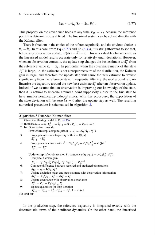
numerical procedure is schematised in Algorithm 3.
Algorithm 3 Extended Kalman filter
Given the filtering model in Eq. (6.73)
1: Initialise t k−1 = t 0 , ¯
x
+
k−1 = ˆ
x
+
k−1 = ˆ
x 0 , P
+
k−1 = P 0 , t k = t 1
2: for Observation times do
Prediction step: compute p(x k |y 1:k−1 ) = N x k (ˆ x
−
k , P
−
k )
3:
Propagate reference trajectory with ˙ ˆ
x = f(t, ¯
x)
¯
x
+
k−1 → ¯
x
−
k
4:
Propagate covariance with ˙
P = ∇ x f
¯
x
P x + P x ∇ x f
T
¯
x
+ GQG T
P
+
k−1 → P
−
k
Update step: after observation ¯
y k compute p(x k |y 1:k ) = N x k (ˆ x
+
k , P
+
k )
5:
Compute Kalman gain
K k = P
−
k ∇ x h
T
¯
x
(∇ x h
¯
x
P
−
k ∇ x h
T
¯
x
+ R k ) −1
6:
Compute difference between received and predicted observations
δ ¯
y k = ¯
y k − h(t k , ¯
x
−
k )
7:
Update deviation mean and state estimate with observation information
δ ¯
x
+
k = K k δ ¯
y k , ˆ
x
+
k = δ ¯
x
+
k + ¯
x
−
k
8:
Update covariance with observation covariance
P
+
k = P
−
k − K k ∇ x h
¯
x
P
−
k
9:
Update quantities for loop iteration
¯
x
+
k−1 = ˆ
x
+
k−1 = ˆ
x
+
k , P
+
k−1 = P
+
k , k = k + 1
10: end for
In the prediction step, the reference trajectory is integrated exactly with the
deterministic terms of the nonlinear dynamics. On the other hand, the linearised
209
δx 0 ∼ N δx 0 (ˆ x 0 − ¯
x 0 , P 0 ) .
(6.77)
This property on the covariance holds at any time P δx = P x because the reference
point ˆ
x is deterministic and fixed. The linearised system can be solved directly with
the Kalman filter.
There is freedom in the choice of the reference point ¯
x 0 , and the obvious choice is
¯
x 0 = ˆ
x 0 . In this case, from Eq. (6.77) and Eq.(6.33), it is straightforward to see that,
before any observation update, E{δx} =
δx = 0. This is a valuable characteristic as
the linearised model results accurate only for relatively small deviations. However,
when an observation comes in, the update step changes the best estimate to ˆ
x
+
k from
the reference value ¯
x k = ˆ
x
−
k . In particular, when the covariance matrix of the state
P
−
k is large, i.e. the estimate is not a proper measure of the distribution, the Kalman
gain is large, and therefore the update step will cause the new estimate to deviate
significantly from the reference state. In sequential filtering, the workaround is to relinearise the trajectory around the new best estimate ˆ
x
+
k after an observation update.
Indeed, if we assume that an observation is improving our knowledge of the state,
then it is natural to linearise around a point supposedly closer to the true state to
have smaller nonlinearity-induced errors. With this procedure, the expectation of
the state deviation will be zero
δx = 0 after the update step as well. The resulting
numerical procedure is schematised in Algorithm 3.
Algorithm 3 Extended Kalman filter
Given the filtering model in Eq. (6.73)
1: Initialise t k−1 = t 0 , ¯
x
+
k−1 = ˆ
x
+
k−1 = ˆ
x 0 , P
+
k−1 = P 0 , t k = t 1
2: for Observation times do
Prediction step: compute p(x k |y 1:k−1 ) = N x k (ˆ x
−
k , P
−
k )
3:
Propagate reference trajectory with ˙ ˆ
x = f(t, ¯
x)
¯
x
+
k−1 → ¯
x
−
k
4:
Propagate covariance with ˙
P = ∇ x f
¯
x
P x + P x ∇ x f
T
¯
x
+ GQG T
P
+
k−1 → P
−
k
Update step: after observation ¯
y k compute p(x k |y 1:k ) = N x k (ˆ x
+
k , P
+
k )
5:
Compute Kalman gain
K k = P
−
k ∇ x h
T
¯
x
(∇ x h
¯
x
P
−
k ∇ x h
T
¯
x
+ R k ) −1
6:
Compute difference between received and predicted observations
δ ¯
y k = ¯
y k − h(t k , ¯
x
−
k )
7:
Update deviation mean and state estimate with observation information
δ ¯
x
+
k = K k δ ¯
y k , ˆ
x
+
k = δ ¯
x
+
k + ¯
x
−
k
8:
Update covariance with observation covariance
P
+
k = P
−
k − K k ∇ x h
¯
x
P
−
k
9:
Update quantities for loop iteration
¯
x
+
k−1 = ˆ
x
+
k−1 = ˆ
x
+
k , P
+
k−1 = P
+
k , k = k + 1
10: end for
In the prediction step, the reference trajectory is integrated exactly with the
deterministic terms of the nonlinear dynamics. On the other hand, the linearised