

6 Fundamentals of Filtering
207
Algorithm 2 Kalman Filter with state transition matrix
Given the filtering model in Eq. (6.57)
1: Initialise t k−1 = t 0 , ˆ
x
+
k−1 = ˆ
x 0 , P
+
k−1 = P 0 , t k = t 1
2: for Observation times do
Prediction step: compute p(x k |y 1:k−1 ) = N x k (ˆ x
−
k , P
−
k )
3:
Propagate state transition matrix ˙
Φ(t, t k−1 ) = F (t)Φ(t, t k−1 )
I → Φ(t k , t k−1 )
4:
Propagate mean estimate
ˆ
x
−
k = Φ(t k , t k−1 )ˆ x
+
k−1
5:
Propagate covariance matrix
P
−
k = Φ(t k , t k−1 )P
+
k−1 Φ T (t k , t k−1 ) + Γ (t k , t k−1 )Q k−1 Γ T (t k , t k−1 )
Update step: after observation ¯
y k compute p(x k |y 1:k ) = N x k (ˆ x
+
k , P
+
k )
6:
Compute Kalman gain
K k = P
−
k H T (H P
−
k H T + R k ) −1
7:
Update mean with observation information
ˆ
x
+
k = ˆ
x
−
k + K k (¯ y k − H ˆ
x
−
k )
8:
Update covariance with observation covariance
P
+
k = P
−
k − K k H P
−
k
9:
Update quantities for loop iteration
ˆ
x
+
k−1 = ˆ
x
+
k , P
+
k−1 = P
+
k , k = k + 1
10: end for
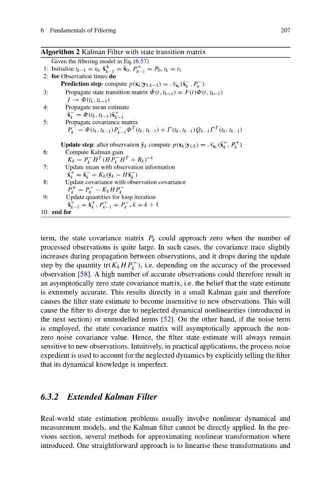
term, the state covariance matrix P k could approach zero when the number of
processed observations is quite large. In such cases, the covariance trace slightly
increases during propagation between observations, and it drops during the update
step by the quantity tr(K k H P
−
k ), i.e. depending on the accuracy of the processed
observation [58]. A high number of accurate observations could therefore result in
an asymptotically zero state covariance matrix, i.e. the belief that the state estimate
is extremely accurate. This results directly in a small Kalman gain and therefore
causes the filter state estimate to become insensitive to new observations. This will
cause the filter to diverge due to neglected dynamical nonlinearities (introduced in
the next section) or unmodelled terms [52]. On the other hand, if the noise term
is employed, the state covariance matrix will asymptotically approach the nonzero noise covariance value. Hence, the filter state estimate will always remain
sensitive to new observations. Intuitively, in practical applications, the process noise
expedient is used to account for the neglected dynamics by explicitly telling the filter
that its dynamical knowledge is imperfect.
6.3.2 Extended Kalman Filter
Real-world state estimation problems usually involve nonlinear dynamical and
measurement models, and the Kalman filter cannot be directly applied. In the previous section, several methods for approximating nonlinear transformation where
introduced. One straightforward approach is to linearise these transformations and
207
Algorithm 2 Kalman Filter with state transition matrix
Given the filtering model in Eq. (6.57)
1: Initialise t k−1 = t 0 , ˆ
x
+
k−1 = ˆ
x 0 , P
+
k−1 = P 0 , t k = t 1
2: for Observation times do
Prediction step: compute p(x k |y 1:k−1 ) = N x k (ˆ x
−
k , P
−
k )
3:
Propagate state transition matrix ˙
Φ(t, t k−1 ) = F (t)Φ(t, t k−1 )
I → Φ(t k , t k−1 )
4:
Propagate mean estimate
ˆ
x
−
k = Φ(t k , t k−1 )ˆ x
+
k−1
5:
Propagate covariance matrix
P
−
k = Φ(t k , t k−1 )P
+
k−1 Φ T (t k , t k−1 ) + Γ (t k , t k−1 )Q k−1 Γ T (t k , t k−1 )
Update step: after observation ¯
y k compute p(x k |y 1:k ) = N x k (ˆ x
+
k , P
+
k )
6:
Compute Kalman gain
K k = P
−
k H T (H P
−
k H T + R k ) −1
7:
Update mean with observation information
ˆ
x
+
k = ˆ
x
−
k + K k (¯ y k − H ˆ
x
−
k )
8:
Update covariance with observation covariance
P
+
k = P
−
k − K k H P
−
k
9:
Update quantities for loop iteration
ˆ
x
+
k−1 = ˆ
x
+
k , P
+
k−1 = P
+
k , k = k + 1
10: end for
term, the state covariance matrix P k could approach zero when the number of
processed observations is quite large. In such cases, the covariance trace slightly
increases during propagation between observations, and it drops during the update
step by the quantity tr(K k H P
−
k ), i.e. depending on the accuracy of the processed
observation [58]. A high number of accurate observations could therefore result in
an asymptotically zero state covariance matrix, i.e. the belief that the state estimate
is extremely accurate. This results directly in a small Kalman gain and therefore
causes the filter state estimate to become insensitive to new observations. This will
cause the filter to diverge due to neglected dynamical nonlinearities (introduced in
the next section) or unmodelled terms [52]. On the other hand, if the noise term
is employed, the state covariance matrix will asymptotically approach the nonzero noise covariance value. Hence, the filter state estimate will always remain
sensitive to new observations. Intuitively, in practical applications, the process noise
expedient is used to account for the neglected dynamics by explicitly telling the filter
that its dynamical knowledge is imperfect.
6.3.2 Extended Kalman Filter
Real-world state estimation problems usually involve nonlinear dynamical and
measurement models, and the Kalman filter cannot be directly applied. In the previous section, several methods for approximating nonlinear transformation where
introduced. One straightforward approach is to linearise these transformations and