

6 Fundamentals of Filtering
201
be advantageous to exploit the previous density π(x 0:k−1 |y 1:k−1 ). The same holds
for the marginal distribution with respect to the current state. For this reason,
sequential filters employ the sequential importance sampling variant [20]. Given
the decomposition of x = x 0:k , the joint target density can be written as the product
of conditional densities as in Eq. (6.10). The importance distribution can be written
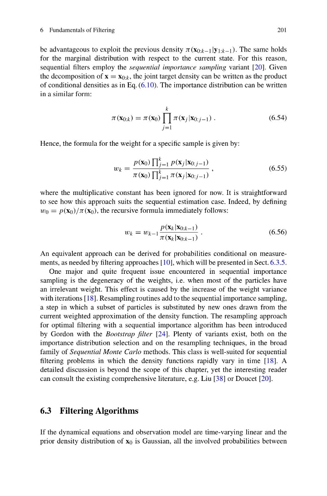
in a similar form:
π(x 0:k ) = π(x 0 )
k
j =1
π(x j |x 0:j −1 ) .
(6.54)
Hence, the formula for the weight for a specific sample is given by:
w k =
p(x 0 )
k
j =1 p(x j |x 0:j −1 )
π(x 0 )
k
j =1 π(x j |x 0:j −1 )
,
(6.55)
where the multiplicative constant has been ignored for now. It is straightforward
to see how this approach suits the sequential estimation case. Indeed, by defining
w 0 = p(x 0 )/π(x 0 ), the recursive formula immediately follows:
w k = w k−1
p(x k |x 0:k−1 )
π(x k |x 0:k−1 )
.
(6.56)
An equivalent approach can be derived for probabilities conditional on measurements, as needed by filtering approaches [10], which will be presented in Sect. 6.3.5.
One major and quite frequent issue encountered in sequential importance
sampling is the degeneracy of the weights, i.e. when most of the particles have
an irrelevant weight. This effect is caused by the increase of the weight variance
with iterations [18]. Resampling routines add to the sequential importance sampling,
a step in which a subset of particles is substituted by new ones drawn from the
current weighted approximation of the density function. The resampling approach
for optimal filtering with a sequential importance algorithm has been introduced
by Gordon with the Bootstrap filter [24]. Plenty of variants exist, both on the
importance distribution selection and on the resampling techniques, in the broad
family of Sequential Monte Carlo methods. This class is well-suited for sequential
filtering problems in which the density functions rapidly vary in time [18]. A
detailed discussion is beyond the scope of this chapter, yet the interesting reader
can consult the existing comprehensive literature, e.g. Liu [38] or Doucet [20].
6.3 Filtering Algorithms
If the dynamical equations and observation model are time-varying linear and the
prior density distribution of x 0 is Gaussian, all the involved probabilities between
201
be advantageous to exploit the previous density π(x 0:k−1 |y 1:k−1 ). The same holds
for the marginal distribution with respect to the current state. For this reason,
sequential filters employ the sequential importance sampling variant [20]. Given
the decomposition of x = x 0:k , the joint target density can be written as the product
of conditional densities as in Eq. (6.10). The importance distribution can be written
in a similar form:
π(x 0:k ) = π(x 0 )
k
j =1
π(x j |x 0:j −1 ) .
(6.54)
Hence, the formula for the weight for a specific sample is given by:
w k =
p(x 0 )
k
j =1 p(x j |x 0:j −1 )
π(x 0 )
k
j =1 π(x j |x 0:j −1 )
,
(6.55)
where the multiplicative constant has been ignored for now. It is straightforward
to see how this approach suits the sequential estimation case. Indeed, by defining
w 0 = p(x 0 )/π(x 0 ), the recursive formula immediately follows:
w k = w k−1
p(x k |x 0:k−1 )
π(x k |x 0:k−1 )
.
(6.56)
An equivalent approach can be derived for probabilities conditional on measurements, as needed by filtering approaches [10], which will be presented in Sect. 6.3.5.
One major and quite frequent issue encountered in sequential importance
sampling is the degeneracy of the weights, i.e. when most of the particles have
an irrelevant weight. This effect is caused by the increase of the weight variance
with iterations [18]. Resampling routines add to the sequential importance sampling,
a step in which a subset of particles is substituted by new ones drawn from the
current weighted approximation of the density function. The resampling approach
for optimal filtering with a sequential importance algorithm has been introduced
by Gordon with the Bootstrap filter [24]. Plenty of variants exist, both on the
importance distribution selection and on the resampling techniques, in the broad
family of Sequential Monte Carlo methods. This class is well-suited for sequential
filtering problems in which the density functions rapidly vary in time [18]. A
detailed discussion is beyond the scope of this chapter, yet the interesting reader
can consult the existing comprehensive literature, e.g. Liu [38] or Doucet [20].
6.3 Filtering Algorithms
If the dynamical equations and observation model are time-varying linear and the
prior density distribution of x 0 is Gaussian, all the involved probabilities between