

194
C. Greco and M. Vasile
6.2 Probability Distribution Propagation
This section will present practical tools for the computation of the evolution of
density functions, presented in the previous theoretical section, when propagated
through arbitrary transformations. In particular, the main difficulty stems from the
general nonlinearity of the dynamical equations f(t, x) and observation relationships
g(t, x). Indeed, in the linear case, the probability propagation has a closed-form
solution, as it will be shown in Sect. 6.2.1. On the other hand, there is no analytical
solution for the general nonlinear case, and approximations shall be introduced to
compute a solution, as shown in Sect. 6.2.2.
6.2.1 Linear Transformation
In the linear time-varying case, the equations describing the evolution of the
distribution moments take a simplified form. Indeed, if the dynamical equations
can be written as
˙
x = F (t)x + G(t)w ,
(6.32)
with w the white Gaussian noise, the Eqs. (6.22) and (6.23) simplify without
approximations to:
d ˆ
x
dt
= F (t)ˆ x
(6.33)
dP x
dt
= F (t)P x + P x F
T (t) + G(t)QG(t)
T ,
(6.34)
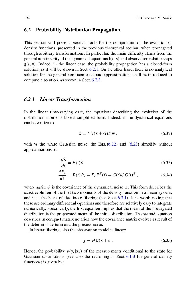
where again Q is the covariance of the dynamical noise w. This form describes the
exact evolution of the first two moments of the density function in a linear system,
and it is the basis of the linear filtering (see Sect. 6.3.1). It is worth noting that
these are ordinary differential equations and therefore are relatively easy to integrate
numerically. Specifically, the first equation implies that the mean of the propagated
distribution is the propagated mean of the initial distribution. The second equation
describes in compact matrix notation how the covariance matrix evolves as result of
the deterministic term and the process noise.
In linear filtering, also the observation model is linear:
y = H (t)x + .
(6.35)
Hence, the probability p(y k |x k ) of the measurements conditional to the state for
Gaussian distributions (see also the reasoning in Sect. 6.1.3 for general density
functions) is given by:
C. Greco and M. Vasile
6.2 Probability Distribution Propagation
This section will present practical tools for the computation of the evolution of
density functions, presented in the previous theoretical section, when propagated
through arbitrary transformations. In particular, the main difficulty stems from the
general nonlinearity of the dynamical equations f(t, x) and observation relationships
g(t, x). Indeed, in the linear case, the probability propagation has a closed-form
solution, as it will be shown in Sect. 6.2.1. On the other hand, there is no analytical
solution for the general nonlinear case, and approximations shall be introduced to
compute a solution, as shown in Sect. 6.2.2.
6.2.1 Linear Transformation
In the linear time-varying case, the equations describing the evolution of the
distribution moments take a simplified form. Indeed, if the dynamical equations
can be written as
˙
x = F (t)x + G(t)w ,
(6.32)
with w the white Gaussian noise, the Eqs. (6.22) and (6.23) simplify without
approximations to:
d ˆ
x
dt
= F (t)ˆ x
(6.33)
dP x
dt
= F (t)P x + P x F
T (t) + G(t)QG(t)
T ,
(6.34)
where again Q is the covariance of the dynamical noise w. This form describes the
exact evolution of the first two moments of the density function in a linear system,
and it is the basis of the linear filtering (see Sect. 6.3.1). It is worth noting that
these are ordinary differential equations and therefore are relatively easy to integrate
numerically. Specifically, the first equation implies that the mean of the propagated
distribution is the propagated mean of the initial distribution. The second equation
describes in compact matrix notation how the covariance matrix evolves as result of
the deterministic term and the process noise.
In linear filtering, also the observation model is linear:
y = H (t)x + .
(6.35)
Hence, the probability p(y k |x k ) of the measurements conditional to the state for
Gaussian distributions (see also the reasoning in Sect. 6.1.3 for general density
functions) is given by: