

192
C. Greco and M. Vasile
Generally, this complete solution is not obtainable; hence a finite-dimensional
approximation is sought. Furthermore, for many practical applications, a single best
estimate, approximating the true state, is required out of the posterior distribution.
Intuitive choices for this statistical estimator could be the posterior’s expectation,
mode, median or any other statistical quantity that is faithfully representative of the
true state in the statistical sense. To formalise this decision process, a loss function
is defined as a real-value function L( x k ) quantifying a penalty (or gain) of choosing
an estimate ˆ
x k rather than another when approximating the true state x k . Ideally, x k
is the deviation from the true state x k = x k −x k , which however is unknown. Hence,
it will be used to denote deviations from the estimate:
x k x k − ˆ
x k .
(6.25)
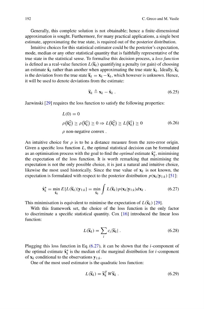
Jazwinski [29] requires the loss function to satisfy the following properties:
L(0) = 0
ρ
x
2
k
≥ ρ
x
1
k
≥ 0 ⇒ L
x
2
k
≥ L
x
1
k
≥ 0
ρ non-negative convex .
(6.26)
An intuitive choice for ρ is to be a distance measure from the zero-error origin.
Given a specific loss function L, the optimal statistical decision can be formulated
as an optimisation process with the goal to find the optimal estimate ˆ
x ∗
k , minimising
the expectation of the loss function. It is worth remarking that minimising the
expectation is not the only possible choice, it is just a natural and intuitive choice,
likewise the most used historically. Since the true value of x k is not known, the
expectation is formulated with respect to the posterior distribution p(x k |y 1:k ) [51]:
ˆ
x
∗
k = min
ˆ
x k
E{L( x k )|y 1:k } = min
ˆ
x k
L( x k )p(x k |y 1:k )dx k .
(6.27)
This minimisation is equivalent to minimise the expectation of L( x k ) [29].
With this framework set, the choice of the loss function is the only factor
to discriminate a specific statistical quantity. Cox [16] introduced the linear loss
function:
L( x k ) =
i
c i | x k | .
(6.28)
Plugging this loss function in Eq. (6.27), it can be shown that the i-component of
the optimal estimate ˆ
x ∗
k is the median of the marginal distribution for i-component
of x k conditional to the observations y 1:k .
One of the most used estimator is the quadratic loss function:
L( x k ) = x
T
k W x k .
(6.29)
C. Greco and M. Vasile
Generally, this complete solution is not obtainable; hence a finite-dimensional
approximation is sought. Furthermore, for many practical applications, a single best
estimate, approximating the true state, is required out of the posterior distribution.
Intuitive choices for this statistical estimator could be the posterior’s expectation,
mode, median or any other statistical quantity that is faithfully representative of the
true state in the statistical sense. To formalise this decision process, a loss function
is defined as a real-value function L( x k ) quantifying a penalty (or gain) of choosing
an estimate ˆ
x k rather than another when approximating the true state x k . Ideally, x k
is the deviation from the true state x k = x k −x k , which however is unknown. Hence,
it will be used to denote deviations from the estimate:
x k x k − ˆ
x k .
(6.25)
Jazwinski [29] requires the loss function to satisfy the following properties:
L(0) = 0
ρ
x
2
k
≥ ρ
x
1
k
≥ 0 ⇒ L
x
2
k
≥ L
x
1
k
≥ 0
ρ non-negative convex .
(6.26)
An intuitive choice for ρ is to be a distance measure from the zero-error origin.
Given a specific loss function L, the optimal statistical decision can be formulated
as an optimisation process with the goal to find the optimal estimate ˆ
x ∗
k , minimising
the expectation of the loss function. It is worth remarking that minimising the
expectation is not the only possible choice, it is just a natural and intuitive choice,
likewise the most used historically. Since the true value of x k is not known, the
expectation is formulated with respect to the posterior distribution p(x k |y 1:k ) [51]:
ˆ
x
∗
k = min
ˆ
x k
E{L( x k )|y 1:k } = min
ˆ
x k
L( x k )p(x k |y 1:k )dx k .
(6.27)
This minimisation is equivalent to minimise the expectation of L( x k ) [29].
With this framework set, the choice of the loss function is the only factor
to discriminate a specific statistical quantity. Cox [16] introduced the linear loss
function:
L( x k ) =
i
c i | x k | .
(6.28)
Plugging this loss function in Eq. (6.27), it can be shown that the i-component of
the optimal estimate ˆ
x ∗
k is the median of the marginal distribution for i-component
of x k conditional to the observations y 1:k .
One of the most used estimator is the quadratic loss function:
L( x k ) = x
T
k W x k .
(6.29)