

184
C. Greco and M. Vasile
will be hidden, without introducing any restriction, for the sake of clarity.
In state estimation, the interest often lies in the computation of conditional
probability distributions on the propagated state. Section 6.2 will introduce
several approximate methods employed to numerically compute this distribution
from the general dynamics in Eq. (6.1).
• Observation model: a set of nonlinear equations describing how a state is mapped
to the measurements taking into account a noise term modelling the error:
y = h(t, x) + .
(6.2)
In this chapter, the noise is considered to have zero-mean and to be additive for
simplicity, whereas similar derivations can be achieved with non-additive noise
[51].
The deterministic term is employed to compute the error-free predicted
observations (or often called computed observations), an important concept both
in the statistical perspective and in practical algorithm formulation [58]. Real
observations are naturally subject to noise and biases dependent on the particular
type of measurement, which should be modelled as well to provide the filter with
more information on the observation received.
• Initial distribution: the a priori knowledge of the state probability distribution
at the initial time, generally assumed independent of any dynamical or observational noise:
p(x 0 ) .
(6.3)
Once these components are defined, the goal of the estimation process is to compute
the optimal combination of generally conflicting information from dynamical
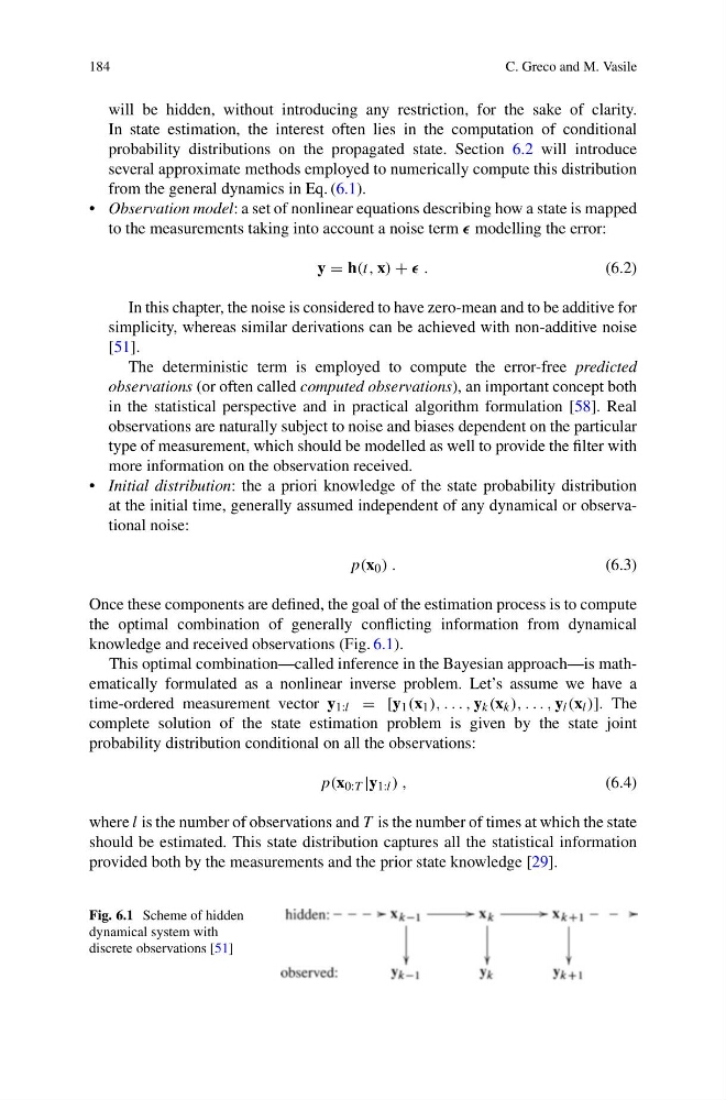
knowledge and received observations (Fig. 6.1).
This optimal combination—called inference in the Bayesian approach—is mathematically formulated as a nonlinear inverse problem. Let’s assume we have a
time-ordered measurement vector y 1:l = [y 1 (x 1 ), . . . , y k (x k ), . . . , y l (x l )]. The
complete solution of the state estimation problem is given by the state joint
probability distribution conditional on all the observations:
p(x 0:T |y 1:l ) ,
(6.4)
where l is the number of observations and T is the number of times at which the state
should be estimated. This state distribution captures all the statistical information
provided both by the measurements and the prior state knowledge [29].
Fig. 6.1 Scheme of hidden
dynamical system with
discrete observations [51]
C. Greco and M. Vasile
will be hidden, without introducing any restriction, for the sake of clarity.
In state estimation, the interest often lies in the computation of conditional
probability distributions on the propagated state. Section 6.2 will introduce
several approximate methods employed to numerically compute this distribution
from the general dynamics in Eq. (6.1).
• Observation model: a set of nonlinear equations describing how a state is mapped
to the measurements taking into account a noise term modelling the error:
y = h(t, x) + .
(6.2)
In this chapter, the noise is considered to have zero-mean and to be additive for
simplicity, whereas similar derivations can be achieved with non-additive noise
[51].
The deterministic term is employed to compute the error-free predicted
observations (or often called computed observations), an important concept both
in the statistical perspective and in practical algorithm formulation [58]. Real
observations are naturally subject to noise and biases dependent on the particular
type of measurement, which should be modelled as well to provide the filter with
more information on the observation received.
• Initial distribution: the a priori knowledge of the state probability distribution
at the initial time, generally assumed independent of any dynamical or observational noise:
p(x 0 ) .
(6.3)
Once these components are defined, the goal of the estimation process is to compute
the optimal combination of generally conflicting information from dynamical
knowledge and received observations (Fig. 6.1).
This optimal combination—called inference in the Bayesian approach—is mathematically formulated as a nonlinear inverse problem. Let’s assume we have a
time-ordered measurement vector y 1:l = [y 1 (x 1 ), . . . , y k (x k ), . . . , y l (x l )]. The
complete solution of the state estimation problem is given by the state joint
probability distribution conditional on all the observations:
p(x 0:T |y 1:l ) ,
(6.4)
where l is the number of observations and T is the number of times at which the state
should be estimated. This state distribution captures all the statistical information
provided both by the measurements and the prior state knowledge [29].
Fig. 6.1 Scheme of hidden
dynamical system with
discrete observations [51]