

5 An Introduction to Imprecise Markov Chains
171
As a second important point, we can consider the entire family of transition
matrices T t for all t ∈ R ≥0 . Then this family constitutes a semi-group of transition
matrices, and Q is the generator of this semi-group. Specifically, it holds that
T t+s = T t T s for all t, s ∈ R ≥0 —this is called the semi-group property. Observe
that it is analogous to the result in Proposition 5.2 and that we already used this
property for the matrix T t+Δ when constructing the derivative.
These properties immediately yield a different representation for the matrix
exponential, which will be convenient further on. We omit the proof.
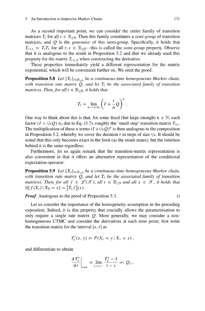
Proposition 5.8 Let {X t } t∈R ≥0 be a continuous-time homogeneous Markov chain,
with transition rate matrix Q, and let T t be the associated family of transition
matrices. Then, for all t ∈ R ≥0 , it holds that
T t = lim
n→+∞
I +
t
n
Q
n
.
One way to think about this is that, for some fixed (but large enough) n ∈ N, each
factor (I + t /nQ) is, due to Eq. (5.7), roughly the ‘small step’ transition matrix Tt /n .
The multiplication of these n terms (I + t /nQ) n is then analogous to the composition
in Proposition 5.2, whereby we cover the duration t in steps of size t /n. It should be
noted that this only becomes exact in the limit (as the result states), but the intuition
behind it is the same regardless.
Furthermore, let us again remark that the transition-matrix representation is
also convenient in that it offers an alternative representation of the conditional
expectation operator:
Proposition 5.9 Let {X t } t∈R ≥0 be a continuous-time homogeneous Markov chain,
with transition rate matrix Q, and let T t be the associated family of transition
matrices. Then, for all f ∈ L (X ), all t ∈ R ≥0 and all x ∈ X , it holds that
E[f (X t ) | X 0 = x] =
T t f
(x) .
Proof Analogous to the proof of Proposition 5.3.
Let us consider the importance of the homogeneity assumption in the preceding
exposition. Indeed, it is this property that crucially allows the parametrisation to
only require a single rate matrix Q. More generally, we may consider a nonhomogeneous CTMC and consider the derivatives at each time point; first write
the transition matrix for the interval [s, t] as
T
t
s (x, y) := P (X t = y | X s = x) ,
and differentiate to obtain
d T t
s
d t
t=s
= lim
t→s +
T t
s − I
t − s
=: Q s ,
171
As a second important point, we can consider the entire family of transition
matrices T t for all t ∈ R ≥0 . Then this family constitutes a semi-group of transition
matrices, and Q is the generator of this semi-group. Specifically, it holds that
T t+s = T t T s for all t, s ∈ R ≥0 —this is called the semi-group property. Observe
that it is analogous to the result in Proposition 5.2 and that we already used this
property for the matrix T t+Δ when constructing the derivative.
These properties immediately yield a different representation for the matrix
exponential, which will be convenient further on. We omit the proof.
Proposition 5.8 Let {X t } t∈R ≥0 be a continuous-time homogeneous Markov chain,
with transition rate matrix Q, and let T t be the associated family of transition
matrices. Then, for all t ∈ R ≥0 , it holds that
T t = lim
n→+∞
I +
t
n
Q
n
.
One way to think about this is that, for some fixed (but large enough) n ∈ N, each
factor (I + t /nQ) is, due to Eq. (5.7), roughly the ‘small step’ transition matrix Tt /n .
The multiplication of these n terms (I + t /nQ) n is then analogous to the composition
in Proposition 5.2, whereby we cover the duration t in steps of size t /n. It should be
noted that this only becomes exact in the limit (as the result states), but the intuition
behind it is the same regardless.
Furthermore, let us again remark that the transition-matrix representation is
also convenient in that it offers an alternative representation of the conditional
expectation operator:
Proposition 5.9 Let {X t } t∈R ≥0 be a continuous-time homogeneous Markov chain,
with transition rate matrix Q, and let T t be the associated family of transition
matrices. Then, for all f ∈ L (X ), all t ∈ R ≥0 and all x ∈ X , it holds that
E[f (X t ) | X 0 = x] =
T t f
(x) .
Proof Analogous to the proof of Proposition 5.3.
Let us consider the importance of the homogeneity assumption in the preceding
exposition. Indeed, it is this property that crucially allows the parametrisation to
only require a single rate matrix Q. More generally, we may consider a nonhomogeneous CTMC and consider the derivatives at each time point; first write
the transition matrix for the interval [s, t] as
T
t
s (x, y) := P (X t = y | X s = x) ,
and differentiate to obtain
d T t
s
d t
t=s
= lim
t→s +
T t
s − I
t − s
=: Q s ,