

164
T. Krak
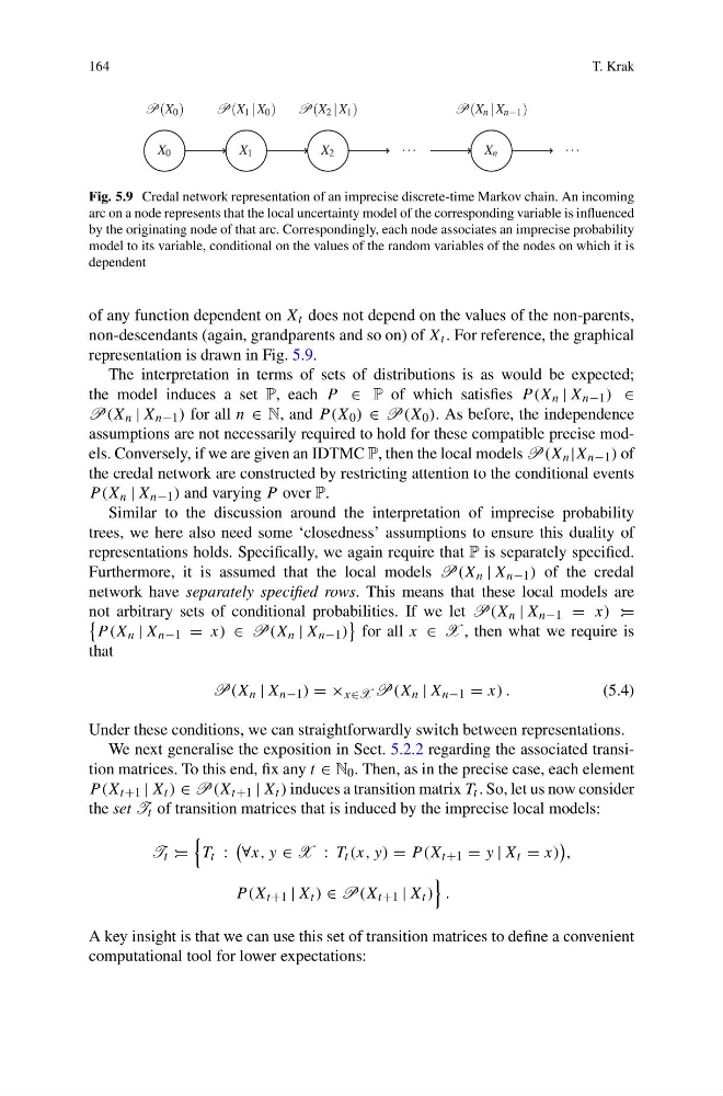
Fig. 5.9 Credal network representation of an imprecise discrete-time Markov chain. An incoming
arc on a node represents that the local uncertainty model of the corresponding variable is influenced
by the originating node of that arc. Correspondingly, each node associates an imprecise probability
model to its variable, conditional on the values of the random variables of the nodes on which it is
dependent
of any function dependent on X t does not depend on the values of the non-parents,
non-descendants (again, grandparents and so on) of X t . For reference, the graphical
representation is drawn in Fig. 5.9.
The interpretation in terms of sets of distributions is as would be expected;
the model induces a set P, each P ∈ P of which satisfies P (X n | X n−1 ) ∈
P(X n | X n−1 ) for all n ∈ N, and P (X 0 ) ∈ P(X 0 ). As before, the independence
assumptions are not necessarily required to hold for these compatible precise models. Conversely, if we are given an IDTMC P, then the local models P(X n |X n−1 ) of
the credal network are constructed by restricting attention to the conditional events
P (X n | X n−1 ) and varying P over P.
Similar to the discussion around the interpretation of imprecise probability
trees, we here also need some ‘closedness’ assumptions to ensure this duality of
representations holds. Specifically, we again require that P is separately specified.
Furthermore, it is assumed that the local models P(X n | X n−1 ) of the credal
network have separately specified rows. This means that these local models are
not arbitrary sets of conditional probabilities. If we let P(X n | X n−1 = x) :=
P (X n | X n−1 = x) ∈ P(X n | X n−1 )
for all x ∈ X , then what we require is
that
P(X n | X n−1 ) = × x∈X P(X n | X n−1 = x) .
(5.4)
Under these conditions, we can straightforwardly switch between representations.
We next generalise the exposition in Sect. 5.2.2 regarding the associated transition matrices. To this end, fix any t ∈ N 0 . Then, as in the precise case, each element
P (X t+1 | X t ) ∈ P(X t+1 | X t ) induces a transition matrix T t . So, let us now consider
the set T t of transition matrices that is induced by the imprecise local models:
T t :=
T t :
∀x, y ∈ X : T t (x, y) = P (X t+1 = y | X t = x)
,
P (X t+1 | X t ) ∈ P(X t+1 | X t )
.
A key insight is that we can use this set of transition matrices to define a convenient
computational tool for lower expectations:
T. Krak
Fig. 5.9 Credal network representation of an imprecise discrete-time Markov chain. An incoming
arc on a node represents that the local uncertainty model of the corresponding variable is influenced
by the originating node of that arc. Correspondingly, each node associates an imprecise probability
model to its variable, conditional on the values of the random variables of the nodes on which it is
dependent
of any function dependent on X t does not depend on the values of the non-parents,
non-descendants (again, grandparents and so on) of X t . For reference, the graphical
representation is drawn in Fig. 5.9.
The interpretation in terms of sets of distributions is as would be expected;
the model induces a set P, each P ∈ P of which satisfies P (X n | X n−1 ) ∈
P(X n | X n−1 ) for all n ∈ N, and P (X 0 ) ∈ P(X 0 ). As before, the independence
assumptions are not necessarily required to hold for these compatible precise models. Conversely, if we are given an IDTMC P, then the local models P(X n |X n−1 ) of
the credal network are constructed by restricting attention to the conditional events
P (X n | X n−1 ) and varying P over P.
Similar to the discussion around the interpretation of imprecise probability
trees, we here also need some ‘closedness’ assumptions to ensure this duality of
representations holds. Specifically, we again require that P is separately specified.
Furthermore, it is assumed that the local models P(X n | X n−1 ) of the credal
network have separately specified rows. This means that these local models are
not arbitrary sets of conditional probabilities. If we let P(X n | X n−1 = x) :=
P (X n | X n−1 = x) ∈ P(X n | X n−1 )
for all x ∈ X , then what we require is
that
P(X n | X n−1 ) = × x∈X P(X n | X n−1 = x) .
(5.4)
Under these conditions, we can straightforwardly switch between representations.
We next generalise the exposition in Sect. 5.2.2 regarding the associated transition matrices. To this end, fix any t ∈ N 0 . Then, as in the precise case, each element
P (X t+1 | X t ) ∈ P(X t+1 | X t ) induces a transition matrix T t . So, let us now consider
the set T t of transition matrices that is induced by the imprecise local models:
T t :=
T t :
∀x, y ∈ X : T t (x, y) = P (X t+1 = y | X t = x)
,
P (X t+1 | X t ) ∈ P(X t+1 | X t )
.
A key insight is that we can use this set of transition matrices to define a convenient
computational tool for lower expectations: