

156
T. Krak
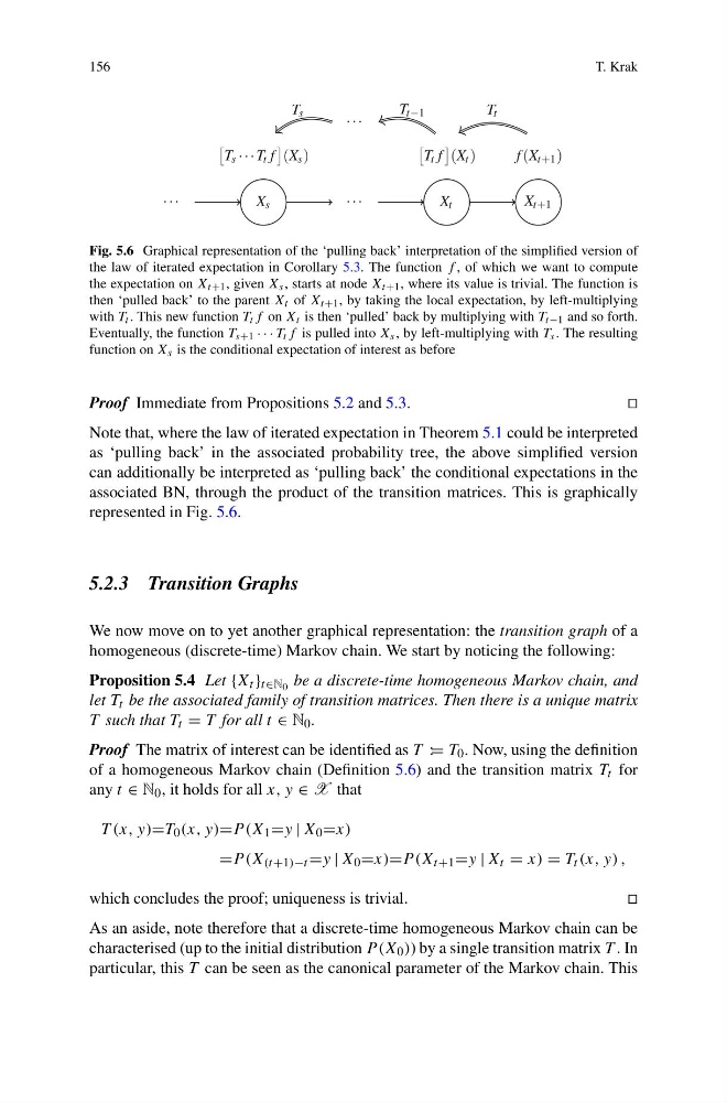
Fig. 5.6 Graphical representation of the ‘pulling back’ interpretation of the simplified version of
the law of iterated expectation in Corollary 5.3. The function f , of which we want to compute
the expectation on X t+1 , given X s , starts at node X t+1 , where its value is trivial. The function is
then ‘pulled back’ to the parent X t of X t+1 , by taking the local expectation, by left-multiplying
with T t . This new function T t f on X t is then ‘pulled’ back by multiplying with T t−1 and so forth.
Eventually, the function T s+1 · · · T t f is pulled into X s , by left-multiplying with T s . The resulting
function on X s is the conditional expectation of interest as before
Proof Immediate from Propositions 5.2 and 5.3.
Note that, where the law of iterated expectation in Theorem 5.1 could be interpreted
as ‘pulling back’ in the associated probability tree, the above simplified version
can additionally be interpreted as ‘pulling back’ the conditional expectations in the
associated BN, through the product of the transition matrices. This is graphically
represented in Fig. 5.6.
5.2.3 Transition Graphs
We now move on to yet another graphical representation: the transition graph of a
homogeneous (discrete-time) Markov chain. We start by noticing the following:
Proposition 5.4 Let {X t } t∈N 0 be a discrete-time homogeneous Markov chain, and
let T t be the associated family of transition matrices. Then there is a unique matrix
T such that T t = T for all t ∈ N 0 .
Proof The matrix of interest can be identified as T := T 0 . Now, using the definition
of a homogeneous Markov chain (Definition 5.6) and the transition matrix T t for
any t ∈ N 0 , it holds for all x, y ∈ X that
T (x, y)=T 0 (x, y)=P (X 1 =y | X 0 =x)
=P (X (t+1)−t =y | X 0 =x)=P (X t+1 =y | X t = x) = T t (x, y) ,
which concludes the proof; uniqueness is trivial.
As an aside, note therefore that a discrete-time homogeneous Markov chain can be
characterised (up to the initial distribution P (X 0 )) by a single transition matrix T . In
particular, this T can be seen as the canonical parameter of the Markov chain. This
T. Krak
Fig. 5.6 Graphical representation of the ‘pulling back’ interpretation of the simplified version of
the law of iterated expectation in Corollary 5.3. The function f , of which we want to compute
the expectation on X t+1 , given X s , starts at node X t+1 , where its value is trivial. The function is
then ‘pulled back’ to the parent X t of X t+1 , by taking the local expectation, by left-multiplying
with T t . This new function T t f on X t is then ‘pulled’ back by multiplying with T t−1 and so forth.
Eventually, the function T s+1 · · · T t f is pulled into X s , by left-multiplying with T s . The resulting
function on X s is the conditional expectation of interest as before
Proof Immediate from Propositions 5.2 and 5.3.
Note that, where the law of iterated expectation in Theorem 5.1 could be interpreted
as ‘pulling back’ in the associated probability tree, the above simplified version
can additionally be interpreted as ‘pulling back’ the conditional expectations in the
associated BN, through the product of the transition matrices. This is graphically
represented in Fig. 5.6.
5.2.3 Transition Graphs
We now move on to yet another graphical representation: the transition graph of a
homogeneous (discrete-time) Markov chain. We start by noticing the following:
Proposition 5.4 Let {X t } t∈N 0 be a discrete-time homogeneous Markov chain, and
let T t be the associated family of transition matrices. Then there is a unique matrix
T such that T t = T for all t ∈ N 0 .
Proof The matrix of interest can be identified as T := T 0 . Now, using the definition
of a homogeneous Markov chain (Definition 5.6) and the transition matrix T t for
any t ∈ N 0 , it holds for all x, y ∈ X that
T (x, y)=T 0 (x, y)=P (X 1 =y | X 0 =x)
=P (X (t+1)−t =y | X 0 =x)=P (X t+1 =y | X t = x) = T t (x, y) ,
which concludes the proof; uniqueness is trivial.
As an aside, note therefore that a discrete-time homogeneous Markov chain can be
characterised (up to the initial distribution P (X 0 )) by a single transition matrix T . In
particular, this T can be seen as the canonical parameter of the Markov chain. This