

150
T. Krak
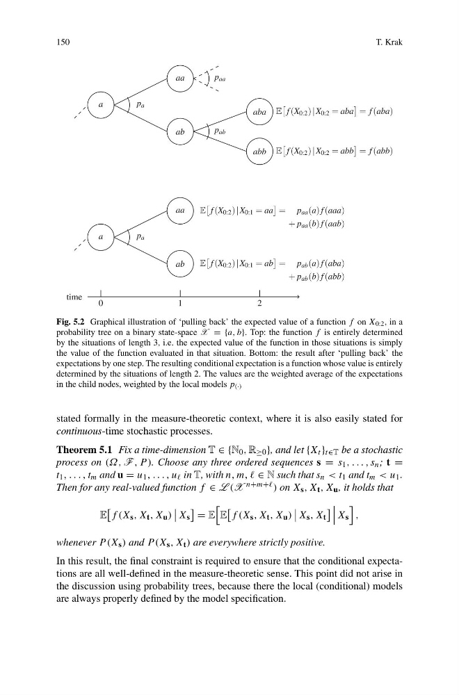
Fig. 5.2 Graphical illustration of ‘pulling back’ the expected value of a function f on X 0:2 , in a
probability tree on a binary state-space X = {a, b}. Top: the function f is entirely determined
by the situations of length 3, i.e. the expected value of the function in those situations is simply
the value of the function evaluated in that situation. Bottom: the result after ‘pulling back’ the
expectations by one step. The resulting conditional expectation is a function whose value is entirely
determined by the situations of length 2. The values are the weighted average of the expectations
in the child nodes, weighted by the local models p (·)
stated formally in the measure-theoretic context, where it is also easily stated for
continuous-time stochastic processes.
Theorem 5.1 Fix a time-dimension T ∈ {N 0 , R ≥0 }, and let {X t } t∈T be a stochastic
process on (Ω, F , P ). Choose any three ordered sequences s = s 1 , . . . , s n ; t =
t 1 , . . . , t m and u = u 1 , . . . , u in T, with n, m, , ∈ N such that s n < t 1 and t m < u 1 .
Then for any real-valued function f ∈ L (X n+m+ ) on X s , X t , X u , it holds that
E
f (X s , X t , X u )
X s
= E
E
f (X s , X t , X u )
X s , X t
X s
,
whenever P (X s ) and P (X s , X t ) are everywhere strictly positive.
In this result, the final constraint is required to ensure that the conditional expectations are all well-defined in the measure-theoretic sense. This point did not arise in
the discussion using probability trees, because there the local (conditional) models
are always properly defined by the model specification.
T. Krak
Fig. 5.2 Graphical illustration of ‘pulling back’ the expected value of a function f on X 0:2 , in a
probability tree on a binary state-space X = {a, b}. Top: the function f is entirely determined
by the situations of length 3, i.e. the expected value of the function in those situations is simply
the value of the function evaluated in that situation. Bottom: the result after ‘pulling back’ the
expectations by one step. The resulting conditional expectation is a function whose value is entirely
determined by the situations of length 2. The values are the weighted average of the expectations
in the child nodes, weighted by the local models p (·)
stated formally in the measure-theoretic context, where it is also easily stated for
continuous-time stochastic processes.
Theorem 5.1 Fix a time-dimension T ∈ {N 0 , R ≥0 }, and let {X t } t∈T be a stochastic
process on (Ω, F , P ). Choose any three ordered sequences s = s 1 , . . . , s n ; t =
t 1 , . . . , t m and u = u 1 , . . . , u in T, with n, m, , ∈ N such that s n < t 1 and t m < u 1 .
Then for any real-valued function f ∈ L (X n+m+ ) on X s , X t , X u , it holds that
E
f (X s , X t , X u )
X s
= E
E
f (X s , X t , X u )
X s , X t
X s
,
whenever P (X s ) and P (X s , X t ) are everywhere strictly positive.
In this result, the final constraint is required to ensure that the conditional expectations are all well-defined in the measure-theoretic sense. This point did not arise in
the discussion using probability trees, because there the local (conditional) models
are always properly defined by the model specification.